Training a Classifier

Created On: Mar 24, 2017 | Last Updated: Dec 20, 2024 | Last Verified: Not Verified

This is it. You have seen how to define neural networks, compute loss and make updates to the weights of the network.

Now you might be thinking,

What about data?

Generally, when you have to deal with image, text, audio or video data, you can use standard python packages that load data into a numpy array. Then you can convert this array into a torch.*Tensor.

• For images, packages such as Pillow, OpenCV are useful

• For audio, packages such as scipy and librosa

• For text, either raw Python or Cython based loading, or NLTK and SpaCy are useful

Specifically for vision, we have created a package called torchvision, that has data loaders for common datasets such as ImageNet, CIFAR10, MNIST, etc. and data transformers for images, viz., torchvision.datasets and torch.utils.data.DataLoader.

This provides a huge convenience and avoids writing boilerplate code.

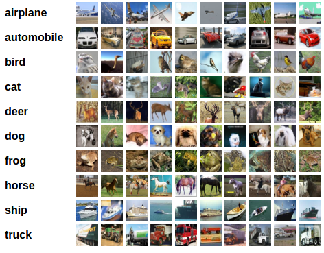
For this tutorial, we will use the CIFAR10 dataset. It has the classes: ‘airplane’, ‘automobile’, ‘bird’, ‘cat’, ‘deer’, ‘dog’, ‘frog’, ‘horse’, ‘ship’, ‘truck’. The images in CIFAR-10 are of size 3x32x32, i.e. 3-channel color images of 32x32 pixels in size.

cifar10

Training an image classifier

We will do the following steps in order:

1. Load and normalize the CIFAR10 training and test datasets using torchvision

2. Define a Convolutional Neural Network

3. Define a loss function

4. Train the network on the training data

5. Test the network on the test data

1. Load and normalize CIFAR10

Using torchvision, it’s extremely easy to load CIFAR10.

import torch
import torchvision
import torchvision.transforms as transforms

The output of torchvision datasets are PILImage images of range [0, 1]. We transform them to Tensors of normalized range [-1, 1].

Note

If running on Windows and you get a BrokenPipeError, try setting the num_worker of torch.utils.data.DataLoader() to 0.

transform = transforms.Compose(
    [transforms.ToTensor(),
     transforms.Normalize((0.5, 0.5, 0.5), (0.5, 0.5, 0.5))])

batch_size = 4

trainset = torchvision.datasets.CIFAR10(root='./data', train=True,
                                        download=True, transform=transform)
trainloader = torch.utils.data.DataLoader(trainset, batch_size=batch_size,
                                          shuffle=True, num_workers=2)

testset = torchvision.datasets.CIFAR10(root='./data', train=False,
                                       download=True, transform=transform)
testloader = torch.utils.data.DataLoader(testset, batch_size=batch_size,
                                         shuffle=False, num_workers=2)

classes = ('plane', 'car', 'bird', 'cat',
           'deer', 'dog', 'frog', 'horse', 'ship', 'truck')

Downloading https://www.cs.toronto.edu/~kriz/cifar-10-python.tar.gz to ./data/cifar-10-python.tar.gz

  0%|          | 0.00/170M [00:00<?, ?B/s]
  0%|          | 524k/170M [00:00<00:32, 5.23MB/s]
  5%|4         | 8.13M/170M [00:00<00:03, 46.8MB/s]
 11%|#1        | 19.0M/170M [00:00<00:02, 74.9MB/s]
 18%|#7        | 29.9M/170M [00:00<00:01, 88.4MB/s]
 24%|##3       | 40.8M/170M [00:00<00:01, 95.9MB/s]
 30%|###       | 51.7M/170M [00:00<00:01, 100MB/s]
 37%|###6      | 62.7M/170M [00:00<00:01, 103MB/s]
 43%|####3     | 73.4M/170M [00:00<00:00, 104MB/s]
 49%|####9     | 83.9M/170M [00:00<00:00, 104MB/s]
 55%|#####5    | 94.3M/170M [00:01<00:00, 103MB/s]
 61%|######1   | 105M/170M [00:01<00:00, 101MB/s]
 68%|######7   | 116M/170M [00:01<00:00, 103MB/s]
 74%|#######4  | 127M/170M [00:01<00:00, 105MB/s]
 81%|########  | 137M/170M [00:01<00:00, 106MB/s]
 87%|########6 | 148M/170M [00:01<00:00, 107MB/s]
 93%|#########3| 159M/170M [00:01<00:00, 108MB/s]
100%|#########9| 170M/170M [00:01<00:00, 108MB/s]
100%|##########| 170M/170M [00:01<00:00, 99.2MB/s]
Extracting ./data/cifar-10-python.tar.gz to ./data
Files already downloaded and verified

Let us show some of the training images, for fun.

import matplotlib.pyplot as plt
import numpy as np

# functions to show an image


def imshow(img):
    img = img / 2 + 0.5     # unnormalize
    npimg = img.numpy()
    plt.imshow(np.transpose(npimg, (1, 2, 0)))
    plt.show()


# get some random training images
dataiter = iter(trainloader)
images, labels = next(dataiter)

# show images
imshow(torchvision.utils.make_grid(images))
# print labels
print(' '.join(f'{classes[labels[j]]:5s}' for j in range(batch_size)))

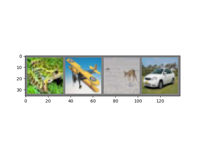
frog  plane deer  car

2. Define a Convolutional Neural Network

Copy the neural network from the Neural Networks section before and modify it to take 3-channel images (instead of 1-channel images as it was defined).

import torch.nn as nn
import torch.nn.functional as F


class Net(nn.Module):
    def __init__(self):
        super().__init__()
        self.conv1 = nn.Conv2d(3, 6, 5)
        self.pool = nn.MaxPool2d(2, 2)
        self.conv2 = nn.Conv2d(6, 16, 5)
        self.fc1 = nn.Linear(16 * 5 * 5, 120)
        self.fc2 = nn.Linear(120, 84)
        self.fc3 = nn.Linear(84, 10)

    def forward(self, x):
        x = self.pool(F.relu(self.conv1(x)))
        x = self.pool(F.relu(self.conv2(x)))
        x = torch.flatten(x, 1) # flatten all dimensions except batch
        x = F.relu(self.fc1(x))
        x = F.relu(self.fc2(x))
        x = self.fc3(x)
        return x


net = Net()

3. Define a Loss function and optimizer

Let’s use a Classification Cross-Entropy loss and SGD with momentum.

import torch.optim as optim

criterion = nn.CrossEntropyLoss()
optimizer = optim.SGD(net.parameters(), lr=0.001, momentum=0.9)

4. Train the network

This is when things start to get interesting. We simply have to loop over our data iterator, and feed the inputs to the network and optimize.

for epoch in range(2):  # loop over the dataset multiple times

    running_loss = 0.0
    for i, data in enumerate(trainloader, 0):
        # get the inputs; data is a list of [inputs, labels]
        inputs, labels = data

        # zero the parameter gradients
        optimizer.zero_grad()

        # forward + backward + optimize
        outputs = net(inputs)
        loss = criterion(outputs, labels)
        loss.backward()
        optimizer.step()

        # print statistics
        running_loss += loss.item()
        if i % 2000 == 1999:    # print every 2000 mini-batches
            print(f'[{epoch + 1}, {i + 1:5d}] loss: {running_loss / 2000:.3f}')
            running_loss = 0.0

print('Finished Training')

[1,  2000] loss: 2.144
[1,  4000] loss: 1.835
[1,  6000] loss: 1.677
[1,  8000] loss: 1.573
[1, 10000] loss: 1.526
[1, 12000] loss: 1.447
[2,  2000] loss: 1.405
[2,  4000] loss: 1.363
[2,  6000] loss: 1.341
[2,  8000] loss: 1.340
[2, 10000] loss: 1.315
[2, 12000] loss: 1.281
Finished Training

Let’s quickly save our trained model:

PATH = './cifar_net.pth'
torch.save(net.state_dict(), PATH)

See here for more details on saving PyTorch models.

5. Test the network on the test data

We have trained the network for 2 passes over the training dataset. But we need to check if the network has learnt anything at all.

We will check this by predicting the class label that the neural network outputs, and checking it against the ground-truth. If the prediction is correct, we add the sample to the list of correct predictions.

Okay, first step. Let us display an image from the test set to get familiar.

dataiter = iter(testloader)
images, labels = next(dataiter)

# print images
imshow(torchvision.utils.make_grid(images))
print('GroundTruth: ', ' '.join(f'{classes[labels[j]]:5s}' for j in range(4)))

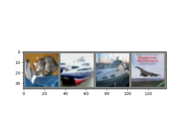
GroundTruth:  cat   ship  ship  plane

Next, let’s load back in our saved model (note: saving and re-loading the model wasn’t necessary here, we only did it to illustrate how to do so):

net = Net()
net.load_state_dict(torch.load(PATH, weights_only=True))

<All keys matched successfully>

Okay, now let us see what the neural network thinks these examples above are:

outputs = net(images)

The outputs are energies for the 10 classes. The higher the energy for a class, the more the network thinks that the image is of the particular class. So, let’s get the index of the highest energy:

_, predicted = torch.max(outputs, 1)

print('Predicted: ', ' '.join(f'{classes[predicted[j]]:5s}'
                              for j in range(4)))

Predicted:  cat   ship  truck ship

The results seem pretty good.

Let us look at how the network performs on the whole dataset.

correct = 0
total = 0
# since we're not training, we don't need to calculate the gradients for our outputs
with torch.no_grad():
    for data in testloader:
        images, labels = data
        # calculate outputs by running images through the network
        outputs = net(images)
        # the class with the highest energy is what we choose as prediction
        _, predicted = torch.max(outputs, 1)
        total += labels.size(0)
        correct += (predicted == labels).sum().item()

print(f'Accuracy of the network on the 10000 test images: {100 * correct // total} %')

Accuracy of the network on the 10000 test images: 54 %

That looks way better than chance, which is 10% accuracy (randomly picking a class out of 10 classes). Seems like the network learnt something.

Hmmm, what are the classes that performed well, and the classes that did not perform well:

# prepare to count predictions for each class
correct_pred = {classname: 0 for classname in classes}
total_pred = {classname: 0 for classname in classes}

# again no gradients needed
with torch.no_grad():
    for data in testloader:
        images, labels = data
        outputs = net(images)
        _, predictions = torch.max(outputs, 1)
        # collect the correct predictions for each class
        for label, prediction in zip(labels, predictions):
            if label == prediction:
                correct_pred[classes[label]] += 1
            total_pred[classes[label]] += 1


# print accuracy for each class
for classname, correct_count in correct_pred.items():
    accuracy = 100 * float(correct_count) / total_pred[classname]
    print(f'Accuracy for class: {classname:5s} is {accuracy:.1f} %')

Accuracy for class: plane is 37.9 %
Accuracy for class: car   is 62.2 %
Accuracy for class: bird  is 45.6 %
Accuracy for class: cat   is 29.2 %
Accuracy for class: deer  is 50.3 %
Accuracy for class: dog   is 45.9 %
Accuracy for class: frog  is 60.1 %
Accuracy for class: horse is 70.3 %
Accuracy for class: ship  is 82.9 %
Accuracy for class: truck is 63.1 %

Okay, so what next?

How do we run these neural networks on the GPU?

Training on GPU

Just like how you transfer a Tensor onto the GPU, you transfer the neural net onto the GPU.

Let’s first define our device as the first visible cuda device if we have CUDA available:

device = torch.device('cuda:0' if torch.cuda.is_available() else 'cpu')

# Assuming that we are on a CUDA machine, this should print a CUDA device:

print(device)

cuda:0

The rest of this section assumes that device is a CUDA device.

Then these methods will recursively go over all modules and convert their parameters and buffers to CUDA tensors:

net.to(device)

Remember that you will have to send the inputs and targets at every step to the GPU too:

inputs, labels = data[0].to(device), data[1].to(device)

Why don’t I notice MASSIVE speedup compared to CPU? Because your network is really small.

Exercise: Try increasing the width of your network (argument 2 of the first nn.Conv2d, and argument 1 of the second nn.Conv2d – they need to be the same number), see what kind of speedup you get.

Goals achieved:

• Understanding PyTorch’s Tensor library and neural networks at a high level.

• Train a small neural network to classify images

Training on multiple GPUs

If you want to see even more MASSIVE speedup using all of your GPUs, please check out Optional: Data Parallelism.

Where do I go next?

• Train neural nets to play video games

• Train a state-of-the-art ResNet network on imagenet

• Train a face generator using Generative Adversarial Networks

• Train a word-level language model using Recurrent LSTM networks

• More examples

• More tutorials

• Discuss PyTorch on the Forums

• Chat with other users on Slack

del dataiter