CTC forced alignment API tutorial

Author: Xiaohui Zhang, Moto Hira

The forced alignment is a process to align transcript with speech. This tutorial shows how to align transcripts to speech using torchaudio.functional.forced_align() which was developed along the work of Scaling Speech Technology to 1,000+ Languages.

forced_align() has custom CPU and CUDA implementations which are more performant than the vanilla Python implementation above, and are more accurate. It can also handle missing transcript with special <star> token.

There is also a high-level API, torchaudio.pipelines.Wav2Vec2FABundle, which wraps the pre/post-processing explained in this tutorial and makes it easy to run forced-alignments. Forced alignment for multilingual data uses this API to illustrate how to align non-English transcripts.

Preparation

import torch
import torchaudio

print(torch.__version__)
print(torchaudio.__version__)

2.6.0.dev20241104
2.5.0.dev20241105

device = torch.device("cuda" if torch.cuda.is_available() else "cpu")
print(device)

cuda

import IPython
import matplotlib.pyplot as plt

import torchaudio.functional as F

First we prepare the speech data and the transcript we area going to use.

SPEECH_FILE = torchaudio.utils.download_asset("tutorial-assets/Lab41-SRI-VOiCES-src-sp0307-ch127535-sg0042.wav")
waveform, _ = torchaudio.load(SPEECH_FILE)
TRANSCRIPT = "i had that curiosity beside me at this moment".split()

Generating emissions

forced_align() takes emission and token sequences and outputs timestaps of the tokens and their scores.

Emission reperesents the frame-wise probability distribution over tokens, and it can be obtained by passing waveform to an acoustic model.

Tokens are numerical expression of transcripts. There are many ways to tokenize transcripts, but here, we simply map alphabets into integer, which is how labels were constructed when the acoustice model we are going to use was trained.

We will use a pre-trained Wav2Vec2 model, torchaudio.pipelines.MMS_FA, to obtain emission and tokenize the transcript.

bundle = torchaudio.pipelines.MMS_FA

model = bundle.get_model(with_star=False).to(device)
with torch.inference_mode():
    emission, _ = model(waveform.to(device))

Downloading: "https://dl.fbaipublicfiles.com/mms/torchaudio/ctc_alignment_mling_uroman/model.pt" to /root/.cache/torch/hub/checkpoints/model.pt

  0%|          | 0.00/1.18G [00:00<?, ?B/s]
  1%|          | 11.9M/1.18G [00:00<00:10, 115MB/s]
  2%|1         | 22.9M/1.18G [00:00<00:14, 87.3MB/s]
  3%|2         | 31.6M/1.18G [00:00<00:15, 77.8MB/s]
  4%|4         | 50.0M/1.18G [00:00<00:10, 114MB/s]
  6%|5         | 67.5M/1.18G [00:00<00:08, 136MB/s]
  7%|6         | 83.1M/1.18G [00:00<00:08, 145MB/s]
  8%|8         | 101M/1.18G [00:00<00:07, 159MB/s]
 10%|9         | 117M/1.18G [00:00<00:08, 130MB/s]
 11%|#         | 131M/1.18G [00:01<00:09, 122MB/s]
 12%|#2        | 145M/1.18G [00:01<00:08, 128MB/s]
 14%|#3        | 162M/1.18G [00:01<00:07, 143MB/s]
 15%|#5        | 182M/1.18G [00:01<00:06, 159MB/s]
 16%|#6        | 198M/1.18G [00:01<00:07, 150MB/s]
 18%|#7        | 214M/1.18G [00:01<00:06, 157MB/s]
 19%|#9        | 230M/1.18G [00:01<00:06, 160MB/s]
 20%|##        | 246M/1.18G [00:01<00:06, 158MB/s]
 22%|##1       | 261M/1.18G [00:01<00:06, 157MB/s]
 23%|##3       | 277M/1.18G [00:02<00:06, 159MB/s]
 24%|##4       | 292M/1.18G [00:02<00:06, 147MB/s]
 25%|##5       | 307M/1.18G [00:02<00:06, 149MB/s]
 27%|##6       | 324M/1.18G [00:02<00:05, 157MB/s]
 28%|##8       | 340M/1.18G [00:02<00:05, 160MB/s]
 30%|##9       | 356M/1.18G [00:02<00:06, 145MB/s]
 31%|###       | 372M/1.18G [00:02<00:05, 150MB/s]
 32%|###2      | 388M/1.18G [00:02<00:05, 147MB/s]
 34%|###3      | 407M/1.18G [00:02<00:05, 160MB/s]
 36%|###5      | 429M/1.18G [00:03<00:04, 180MB/s]
 37%|###7      | 449M/1.18G [00:03<00:04, 187MB/s]
 39%|###8      | 468M/1.18G [00:03<00:04, 190MB/s]
 40%|####      | 486M/1.18G [00:03<00:03, 189MB/s]
 42%|####1     | 505M/1.18G [00:03<00:03, 191MB/s]
 43%|####3     | 523M/1.18G [00:03<00:03, 182MB/s]
 45%|####4     | 541M/1.18G [00:03<00:04, 158MB/s]
 47%|####6     | 562M/1.18G [00:03<00:03, 175MB/s]
 48%|####8     | 580M/1.18G [00:04<00:04, 147MB/s]
 50%|####9     | 601M/1.18G [00:04<00:03, 165MB/s]
 51%|#####1    | 618M/1.18G [00:04<00:03, 166MB/s]
 53%|#####2    | 636M/1.18G [00:04<00:03, 172MB/s]
 55%|#####4    | 657M/1.18G [00:04<00:03, 185MB/s]
 56%|#####6    | 677M/1.18G [00:04<00:02, 191MB/s]
 58%|#####7    | 697M/1.18G [00:04<00:02, 196MB/s]
 60%|#####9    | 718M/1.18G [00:04<00:02, 201MB/s]
 61%|######1   | 738M/1.18G [00:04<00:02, 200MB/s]
 63%|######2   | 758M/1.18G [00:04<00:02, 203MB/s]
 65%|######4   | 778M/1.18G [00:05<00:02, 195MB/s]
 66%|######6   | 796M/1.18G [00:05<00:02, 157MB/s]
 68%|######7   | 813M/1.18G [00:05<00:02, 154MB/s]
 69%|######9   | 834M/1.18G [00:05<00:02, 172MB/s]
 71%|#######1  | 859M/1.18G [00:05<00:01, 193MB/s]
 73%|#######2  | 878M/1.18G [00:05<00:01, 182MB/s]
 74%|#######4  | 896M/1.18G [00:05<00:01, 173MB/s]
 76%|#######5  | 914M/1.18G [00:05<00:01, 177MB/s]
 77%|#######7  | 931M/1.18G [00:06<00:01, 173MB/s]
 79%|#######8  | 948M/1.18G [00:06<00:01, 162MB/s]
 80%|########  | 967M/1.18G [00:06<00:01, 170MB/s]
 82%|########1 | 984M/1.18G [00:06<00:01, 173MB/s]
 83%|########3 | 0.98G/1.18G [00:06<00:01, 176MB/s]
 85%|########4 | 1.00G/1.18G [00:06<00:01, 162MB/s]
 87%|########6 | 1.02G/1.18G [00:06<00:00, 186MB/s]
 89%|########8 | 1.04G/1.18G [00:06<00:00, 197MB/s]
 90%|######### | 1.06G/1.18G [00:06<00:00, 193MB/s]
 92%|#########1| 1.08G/1.18G [00:06<00:00, 191MB/s]
 93%|#########3| 1.10G/1.18G [00:07<00:00, 194MB/s]
 95%|#########4| 1.11G/1.18G [00:07<00:00, 193MB/s]
 96%|#########6| 1.13G/1.18G [00:07<00:00, 183MB/s]
 98%|#########7| 1.15G/1.18G [00:07<00:00, 176MB/s]
 99%|#########9| 1.17G/1.18G [00:07<00:00, 151MB/s]
100%|##########| 1.18G/1.18G [00:07<00:00, 165MB/s]

def plot_emission(emission):
    fig, ax = plt.subplots()
    ax.imshow(emission.cpu().T)
    ax.set_title("Frame-wise class probabilities")
    ax.set_xlabel("Time")
    ax.set_ylabel("Labels")
    fig.tight_layout()


plot_emission(emission[0])

Tokenize the transcript

We create a dictionary, which maps each label into token.

LABELS = bundle.get_labels(star=None)
DICTIONARY = bundle.get_dict(star=None)
for k, v in DICTIONARY.items():
    print(f"{k}: {v}")

-: 0
a: 1
i: 2
e: 3
n: 4
o: 5
u: 6
t: 7
s: 8
r: 9
m: 10
k: 11
l: 12
d: 13
g: 14
h: 15
y: 16
b: 17
p: 18
w: 19
c: 20
v: 21
j: 22
z: 23
f: 24
': 25
q: 26
x: 27

converting transcript to tokens is as simple as

tokenized_transcript = [DICTIONARY[c] for word in TRANSCRIPT for c in word]

for t in tokenized_transcript:
    print(t, end=" ")
print()

2 15 1 13 7 15 1 7 20 6 9 2 5 8 2 7 16 17 3 8 2 13 3 10 3 1 7 7 15 2 8 10 5 10 3 4 7

Computing alignments

Frame-level alignments

Now we call TorchAudio’s forced alignment API to compute the frame-level alignment. For the detail of function signature, please refer to forced_align().

def align(emission, tokens):
    targets = torch.tensor([tokens], dtype=torch.int32, device=device)
    alignments, scores = F.forced_align(emission, targets, blank=0)

    alignments, scores = alignments[0], scores[0]  # remove batch dimension for simplicity
    scores = scores.exp()  # convert back to probability
    return alignments, scores


aligned_tokens, alignment_scores = align(emission, tokenized_transcript)

Now let’s look at the output.

for i, (ali, score) in enumerate(zip(aligned_tokens, alignment_scores)):
    print(f"{i:3d}:\t{ali:2d} [{LABELS[ali]}], {score:.2f}")

  0:     0 [-], 1.00
  1:     0 [-], 1.00
  2:     0 [-], 1.00
  3:     0 [-], 1.00
  4:     0 [-], 1.00
  5:     0 [-], 1.00
  6:     0 [-], 1.00
  7:     0 [-], 1.00
  8:     0 [-], 1.00
  9:     0 [-], 1.00
 10:     0 [-], 1.00
 11:     0 [-], 1.00
 12:     0 [-], 1.00
 13:     0 [-], 1.00
 14:     0 [-], 1.00
 15:     0 [-], 1.00
 16:     0 [-], 1.00
 17:     0 [-], 1.00
 18:     0 [-], 1.00
 19:     0 [-], 1.00
 20:     0 [-], 1.00
 21:     0 [-], 1.00
 22:     0 [-], 1.00
 23:     0 [-], 1.00
 24:     0 [-], 1.00
 25:     0 [-], 1.00
 26:     0 [-], 1.00
 27:     0 [-], 1.00
 28:     0 [-], 1.00
 29:     0 [-], 1.00
 30:     0 [-], 1.00
 31:     0 [-], 1.00
 32:     2 [i], 1.00
 33:     0 [-], 1.00
 34:     0 [-], 1.00
 35:    15 [h], 1.00
 36:    15 [h], 0.93
 37:     1 [a], 1.00
 38:     0 [-], 0.96
 39:     0 [-], 1.00
 40:     0 [-], 1.00
 41:    13 [d], 1.00
 42:     0 [-], 1.00
 43:     0 [-], 0.97
 44:     7 [t], 1.00
 45:    15 [h], 1.00
 46:     0 [-], 0.98
 47:     1 [a], 1.00
 48:     0 [-], 1.00
 49:     0 [-], 1.00
 50:     7 [t], 1.00
 51:     0 [-], 1.00
 52:     0 [-], 1.00
 53:     0 [-], 1.00
 54:    20 [c], 1.00
 55:     0 [-], 1.00
 56:     0 [-], 1.00
 57:     0 [-], 1.00
 58:     6 [u], 1.00
 59:     6 [u], 0.96
 60:     0 [-], 1.00
 61:     0 [-], 1.00
 62:     0 [-], 0.53
 63:     9 [r], 1.00
 64:     0 [-], 1.00
 65:     2 [i], 1.00
 66:     0 [-], 1.00
 67:     0 [-], 1.00
 68:     0 [-], 1.00
 69:     0 [-], 1.00
 70:     0 [-], 1.00
 71:     0 [-], 0.96
 72:     5 [o], 1.00
 73:     0 [-], 1.00
 74:     0 [-], 1.00
 75:     0 [-], 1.00
 76:     0 [-], 1.00
 77:     0 [-], 1.00
 78:     0 [-], 1.00
 79:     8 [s], 1.00
 80:     0 [-], 1.00
 81:     0 [-], 1.00
 82:     0 [-], 0.99
 83:     2 [i], 1.00
 84:     0 [-], 1.00
 85:     7 [t], 1.00
 86:     0 [-], 1.00
 87:     0 [-], 1.00
 88:    16 [y], 1.00
 89:     0 [-], 1.00
 90:     0 [-], 1.00
 91:     0 [-], 1.00
 92:     0 [-], 1.00
 93:    17 [b], 1.00
 94:     0 [-], 1.00
 95:     3 [e], 1.00
 96:     0 [-], 1.00
 97:     0 [-], 1.00
 98:     0 [-], 1.00
 99:     0 [-], 1.00
100:     0 [-], 1.00
101:     8 [s], 1.00
102:     0 [-], 1.00
103:     0 [-], 1.00
104:     0 [-], 1.00
105:     0 [-], 1.00
106:     0 [-], 1.00
107:     0 [-], 1.00
108:     0 [-], 1.00
109:     0 [-], 0.64
110:     2 [i], 1.00
111:     0 [-], 1.00
112:     0 [-], 1.00
113:    13 [d], 1.00
114:     3 [e], 0.85
115:     0 [-], 1.00
116:    10 [m], 1.00
117:     0 [-], 1.00
118:     0 [-], 1.00
119:     3 [e], 1.00
120:     0 [-], 1.00
121:     0 [-], 1.00
122:     0 [-], 1.00
123:     0 [-], 1.00
124:     1 [a], 1.00
125:     0 [-], 1.00
126:     0 [-], 1.00
127:     7 [t], 1.00
128:     0 [-], 1.00
129:     7 [t], 1.00
130:    15 [h], 1.00
131:     0 [-], 0.79
132:     2 [i], 1.00
133:     0 [-], 1.00
134:     0 [-], 1.00
135:     0 [-], 1.00
136:     8 [s], 1.00
137:     0 [-], 1.00
138:     0 [-], 1.00
139:     0 [-], 1.00
140:     0 [-], 1.00
141:    10 [m], 1.00
142:     0 [-], 1.00
143:     0 [-], 1.00
144:     5 [o], 1.00
145:     0 [-], 1.00
146:     0 [-], 1.00
147:     0 [-], 1.00
148:    10 [m], 1.00
149:     0 [-], 1.00
150:     0 [-], 1.00
151:     3 [e], 1.00
152:     0 [-], 1.00
153:     4 [n], 1.00
154:     0 [-], 1.00
155:     7 [t], 1.00
156:     0 [-], 1.00
157:     0 [-], 1.00
158:     0 [-], 1.00
159:     0 [-], 1.00
160:     0 [-], 1.00
161:     0 [-], 1.00
162:     0 [-], 1.00
163:     0 [-], 1.00
164:     0 [-], 1.00
165:     0 [-], 1.00
166:     0 [-], 1.00
167:     0 [-], 1.00
168:     0 [-], 1.00

Note

The alignment is expressed in the frame cordinate of the emission, which is different from the original waveform.

It contains blank tokens and repeated tokens. The following is the interpretation of the non-blank tokens.

31:     0 [-], 1.00
32:     2 [i], 1.00  "i" starts and ends
33:     0 [-], 1.00
34:     0 [-], 1.00
35:    15 [h], 1.00  "h" starts
36:    15 [h], 0.93  "h" ends
37:     1 [a], 1.00  "a" starts and ends
38:     0 [-], 0.96
39:     0 [-], 1.00
40:     0 [-], 1.00
41:    13 [d], 1.00  "d" starts and ends
42:     0 [-], 1.00

Note

When same token occured after blank tokens, it is not treated as a repeat, but as a new occurrence.

a a a b -> a b
a - - b -> a b
a a - b -> a b
a - a b -> a a b
  ^^^       ^^^

Token-level alignments

Next step is to resolve the repetation, so that each alignment does not depend on previous alignments. torchaudio.functional.merge_tokens() computes the TokenSpan object, which represents which token from the transcript is present at what time span.

token_spans = F.merge_tokens(aligned_tokens, alignment_scores)

print("Token\tTime\tScore")
for s in token_spans:
    print(f"{LABELS[s.token]}\t[{s.start:3d}, {s.end:3d})\t{s.score:.2f}")

Token   Time    Score
i       [ 32,  33)      1.00
h       [ 35,  37)      0.96
a       [ 37,  38)      1.00
d       [ 41,  42)      1.00
t       [ 44,  45)      1.00
h       [ 45,  46)      1.00
a       [ 47,  48)      1.00
t       [ 50,  51)      1.00
c       [ 54,  55)      1.00
u       [ 58,  60)      0.98
r       [ 63,  64)      1.00
i       [ 65,  66)      1.00
o       [ 72,  73)      1.00
s       [ 79,  80)      1.00
i       [ 83,  84)      1.00
t       [ 85,  86)      1.00
y       [ 88,  89)      1.00
b       [ 93,  94)      1.00
e       [ 95,  96)      1.00
s       [101, 102)      1.00
i       [110, 111)      1.00
d       [113, 114)      1.00
e       [114, 115)      0.85
m       [116, 117)      1.00
e       [119, 120)      1.00
a       [124, 125)      1.00
t       [127, 128)      1.00
t       [129, 130)      1.00
h       [130, 131)      1.00
i       [132, 133)      1.00
s       [136, 137)      1.00
m       [141, 142)      1.00
o       [144, 145)      1.00
m       [148, 149)      1.00
e       [151, 152)      1.00
n       [153, 154)      1.00
t       [155, 156)      1.00

Word-level alignments

Now let’s group the token-level alignments into word-level alignments.

def unflatten(list_, lengths):
    assert len(list_) == sum(lengths)
    i = 0
    ret = []
    for l in lengths:
        ret.append(list_[i : i + l])
        i += l
    return ret


word_spans = unflatten(token_spans, [len(word) for word in TRANSCRIPT])

Audio previews

# Compute average score weighted by the span length
def _score(spans):
    return sum(s.score * len(s) for s in spans) / sum(len(s) for s in spans)


def preview_word(waveform, spans, num_frames, transcript, sample_rate=bundle.sample_rate):
    ratio = waveform.size(1) / num_frames
    x0 = int(ratio * spans[0].start)
    x1 = int(ratio * spans[-1].end)
    print(f"{transcript} ({_score(spans):.2f}): {x0 / sample_rate:.3f} - {x1 / sample_rate:.3f} sec")
    segment = waveform[:, x0:x1]
    return IPython.display.Audio(segment.numpy(), rate=sample_rate)


num_frames = emission.size(1)

# Generate the audio for each segment
print(TRANSCRIPT)
IPython.display.Audio(SPEECH_FILE)

['i', 'had', 'that', 'curiosity', 'beside', 'me', 'at', 'this', 'moment']

preview_word(waveform, word_spans[0], num_frames, TRANSCRIPT[0])

i (1.00): 0.644 - 0.664 sec

preview_word(waveform, word_spans[1], num_frames, TRANSCRIPT[1])

had (0.98): 0.704 - 0.845 sec

preview_word(waveform, word_spans[2], num_frames, TRANSCRIPT[2])

that (1.00): 0.885 - 1.026 sec

preview_word(waveform, word_spans[3], num_frames, TRANSCRIPT[3])

curiosity (1.00): 1.086 - 1.790 sec

preview_word(waveform, word_spans[4], num_frames, TRANSCRIPT[4])

beside (0.97): 1.871 - 2.314 sec

preview_word(waveform, word_spans[5], num_frames, TRANSCRIPT[5])

me (1.00): 2.334 - 2.414 sec

preview_word(waveform, word_spans[6], num_frames, TRANSCRIPT[6])

at (1.00): 2.495 - 2.575 sec

preview_word(waveform, word_spans[7], num_frames, TRANSCRIPT[7])

this (1.00): 2.595 - 2.756 sec

preview_word(waveform, word_spans[8], num_frames, TRANSCRIPT[8])

moment (1.00): 2.837 - 3.138 sec

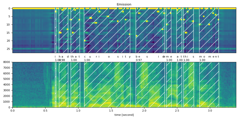
Visualization

Now let’s look at the alignment result and segment the original speech into words.

def plot_alignments(waveform, token_spans, emission, transcript, sample_rate=bundle.sample_rate):
    ratio = waveform.size(1) / emission.size(1) / sample_rate

    fig, axes = plt.subplots(2, 1)
    axes[0].imshow(emission[0].detach().cpu().T, aspect="auto")
    axes[0].set_title("Emission")
    axes[0].set_xticks([])

    axes[1].specgram(waveform[0], Fs=sample_rate)
    for t_spans, chars in zip(token_spans, transcript):
        t0, t1 = t_spans[0].start + 0.1, t_spans[-1].end - 0.1
        axes[0].axvspan(t0 - 0.5, t1 - 0.5, facecolor="None", hatch="/", edgecolor="white")
        axes[1].axvspan(ratio * t0, ratio * t1, facecolor="None", hatch="/", edgecolor="white")
        axes[1].annotate(f"{_score(t_spans):.2f}", (ratio * t0, sample_rate * 0.51), annotation_clip=False)

        for span, char in zip(t_spans, chars):
            t0 = span.start * ratio
            axes[1].annotate(char, (t0, sample_rate * 0.55), annotation_clip=False)

    axes[1].set_xlabel("time [second]")
    axes[1].set_xlim([0, None])
    fig.tight_layout()

plot_alignments(waveform, word_spans, emission, TRANSCRIPT)

Inconsistent treatment of blank token

When splitting the token-level alignments into words, you will notice that some blank tokens are treated differently, and this makes the interpretation of the result somehwat ambigious.

This is easy to see when we plot the scores. The following figure shows word regions and non-word regions, with the frame-level scores of non-blank tokens.

def plot_scores(word_spans, scores):
    fig, ax = plt.subplots()
    span_xs, span_hs = [], []
    ax.axvspan(word_spans[0][0].start - 0.05, word_spans[-1][-1].end + 0.05, facecolor="paleturquoise", edgecolor="none", zorder=-1)
    for t_span in word_spans:
        for span in t_span:
            for t in range(span.start, span.end):
                span_xs.append(t + 0.5)
                span_hs.append(scores[t].item())
            ax.annotate(LABELS[span.token], (span.start, -0.07))
        ax.axvspan(t_span[0].start - 0.05, t_span[-1].end + 0.05, facecolor="mistyrose", edgecolor="none", zorder=-1)
    ax.bar(span_xs, span_hs, color="lightsalmon", edgecolor="coral")
    ax.set_title("Frame-level scores and word segments")
    ax.set_ylim(-0.1, None)
    ax.grid(True, axis="y")
    ax.axhline(0, color="black")
    fig.tight_layout()


plot_scores(word_spans, alignment_scores)

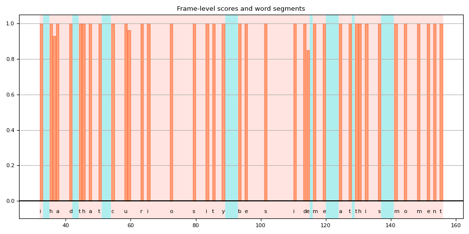
In this plot, the blank tokens are those highlighted area without vertical bar. You can see that there are blank tokens which are interpreted as part of a word (highlighted red), while the others (highlighted blue) are not.

One reason for this is because the model was trained without a label for the word boundary. The blank tokens are treated not just as repeatation but also as silence between words.

But then, a question arises. Should frames immediately after or near the end of a word be silent or repeat?

In the above example, if you go back to the previous plot of spectrogram and word regions, you see that after “y” in “curiosity”, there is still some activities in multiple frequency buckets.

Would it be more accurate if that frame was included in the word?

Unfortunately, CTC does not provide a comprehensive solution to this. Models trained with CTC are known to exhibit “peaky” response, that is, they tend to spike for an aoccurance of a label, but the spike does not last for the duration of the label. (Note: Pre-trained Wav2Vec2 models tend to spike at the beginning of label occurances, but this not always the case.)

[Zeyer et al., 2021] has in-depth alanysis on the peaky behavior of CTC. We encourage those who are interested understanding more to refer to the paper. The following is a quote from the paper, which is the exact issue we are facing here.

Peaky behavior can be problematic in certain cases, e.g. when an application requires to not use the blank label, e.g. to get meaningful time accurate alignments of phonemes to a transcription.

Advanced: Handling transcripts with <star> token

Now let’s look at when the transcript is partially missing, how can we improve alignment quality using the <star> token, which is capable of modeling any token.

Here we use the same English example as used above. But we remove the beginning text “i had that curiosity beside me at” from the transcript. Aligning audio with such transcript results in wrong alignments of the existing word “this”. However, this issue can be mitigated by using the <star> token to model the missing text.

First, we extend the dictionary to include the <star> token.

DICTIONARY["*"] = len(DICTIONARY)

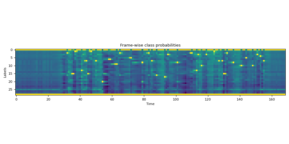
Next, we extend the emission tensor with the extra dimension corresponding to the <star> token.

star_dim = torch.zeros((1, emission.size(1), 1), device=emission.device, dtype=emission.dtype)
emission = torch.cat((emission, star_dim), 2)

assert len(DICTIONARY) == emission.shape[2]

plot_emission(emission[0])

The following function combines all the processes, and compute word segments from emission in one-go.

def compute_alignments(emission, transcript, dictionary):
    tokens = [dictionary[char] for word in transcript for char in word]
    alignment, scores = align(emission, tokens)
    token_spans = F.merge_tokens(alignment, scores)
    word_spans = unflatten(token_spans, [len(word) for word in transcript])
    return word_spans

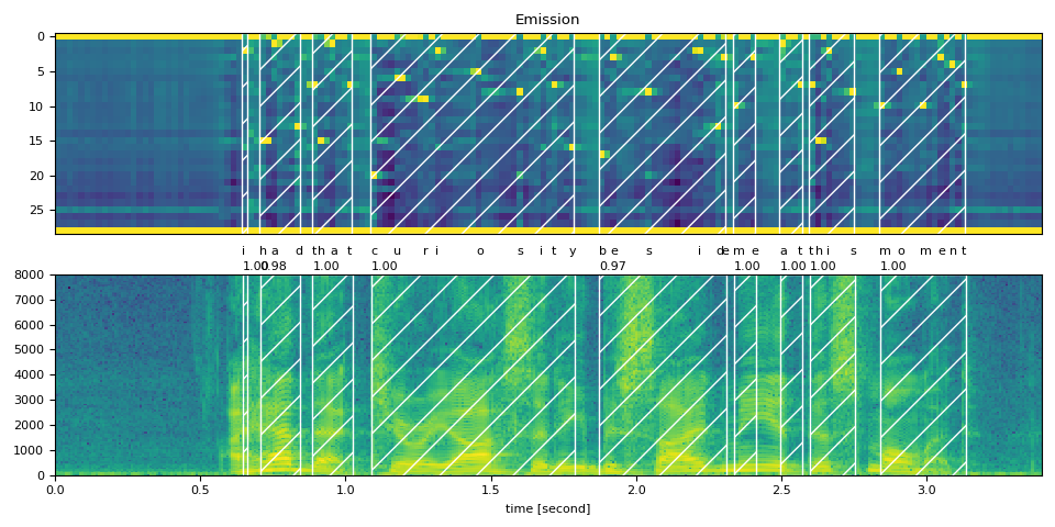
Full Transcript

word_spans = compute_alignments(emission, TRANSCRIPT, DICTIONARY)
plot_alignments(waveform, word_spans, emission, TRANSCRIPT)

Partial Transcript with <star> token

Now we replace the first part of the transcript with the <star> token.

transcript = "* this moment".split()
word_spans = compute_alignments(emission, transcript, DICTIONARY)
plot_alignments(waveform, word_spans, emission, transcript)

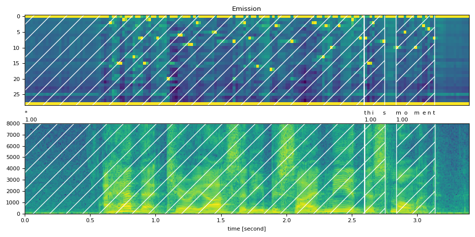
preview_word(waveform, word_spans[0], num_frames, transcript[0])

* (1.00): 0.000 - 2.595 sec

preview_word(waveform, word_spans[1], num_frames, transcript[1])

this (1.00): 2.595 - 2.756 sec

preview_word(waveform, word_spans[2], num_frames, transcript[2])

moment (1.00): 2.837 - 3.138 sec

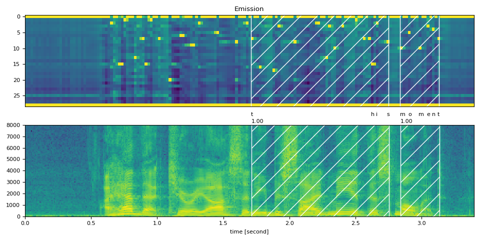
Partial Transcript without <star> token

As a comparison, the following aligns the partial transcript without using <star> token. It demonstrates the effect of <star> token for dealing with deletion errors.

transcript = "this moment".split()
word_spans = compute_alignments(emission, transcript, DICTIONARY)
plot_alignments(waveform, word_spans, emission, transcript)

Conclusion

In this tutorial, we looked at how to use torchaudio’s forced alignment API to align and segment speech files, and demonstrated one advanced usage: How introducing a <star> token could improve alignment accuracy when transcription errors exist.

Acknowledgement

Thanks to Vineel Pratap and Zhaoheng Ni for developing and open-sourcing the forced aligner API.