Audio Feature Extractions

Author: Moto Hira

torchaudio implements feature extractions commonly used in the audio domain. They are available in torchaudio.functional and torchaudio.transforms.

functional implements features as standalone functions. They are stateless.

transforms implements features as objects, using implementations from functional and torch.nn.Module. They can be serialized using TorchScript.

import torch
import torchaudio
import torchaudio.functional as F
import torchaudio.transforms as T

print(torch.__version__)
print(torchaudio.__version__)

import librosa
import matplotlib.pyplot as plt

2.4.0.dev20240416
2.2.0.dev20240418

Overview of audio features

The following diagram shows the relationship between common audio features and torchaudio APIs to generate them.

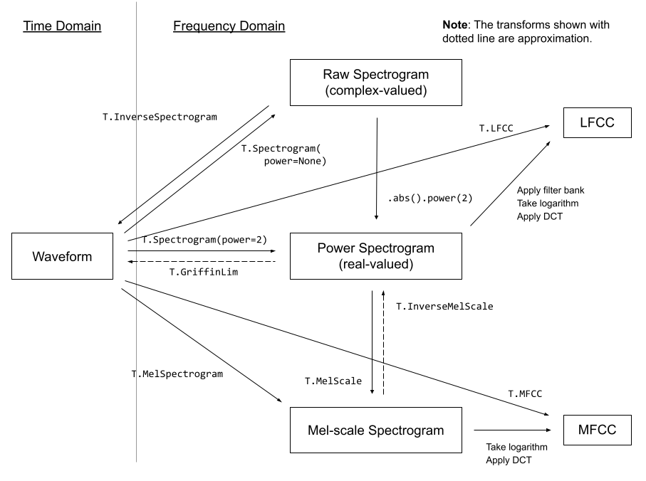
For the complete list of available features, please refer to the documentation.

Preparation

Note

When running this tutorial in Google Colab, install the required packages

!pip install librosa

from IPython.display import Audio
from matplotlib.patches import Rectangle
from torchaudio.utils import download_asset

torch.random.manual_seed(0)

SAMPLE_SPEECH = download_asset("tutorial-assets/Lab41-SRI-VOiCES-src-sp0307-ch127535-sg0042.wav")


def plot_waveform(waveform, sr, title="Waveform", ax=None):
    waveform = waveform.numpy()

    num_channels, num_frames = waveform.shape
    time_axis = torch.arange(0, num_frames) / sr

    if ax is None:
        _, ax = plt.subplots(num_channels, 1)
    ax.plot(time_axis, waveform[0], linewidth=1)
    ax.grid(True)
    ax.set_xlim([0, time_axis[-1]])
    ax.set_title(title)


def plot_spectrogram(specgram, title=None, ylabel="freq_bin", ax=None):
    if ax is None:
        _, ax = plt.subplots(1, 1)
    if title is not None:
        ax.set_title(title)
    ax.set_ylabel(ylabel)
    ax.imshow(librosa.power_to_db(specgram), origin="lower", aspect="auto", interpolation="nearest")


def plot_fbank(fbank, title=None):
    fig, axs = plt.subplots(1, 1)
    axs.set_title(title or "Filter bank")
    axs.imshow(fbank, aspect="auto")
    axs.set_ylabel("frequency bin")
    axs.set_xlabel("mel bin")

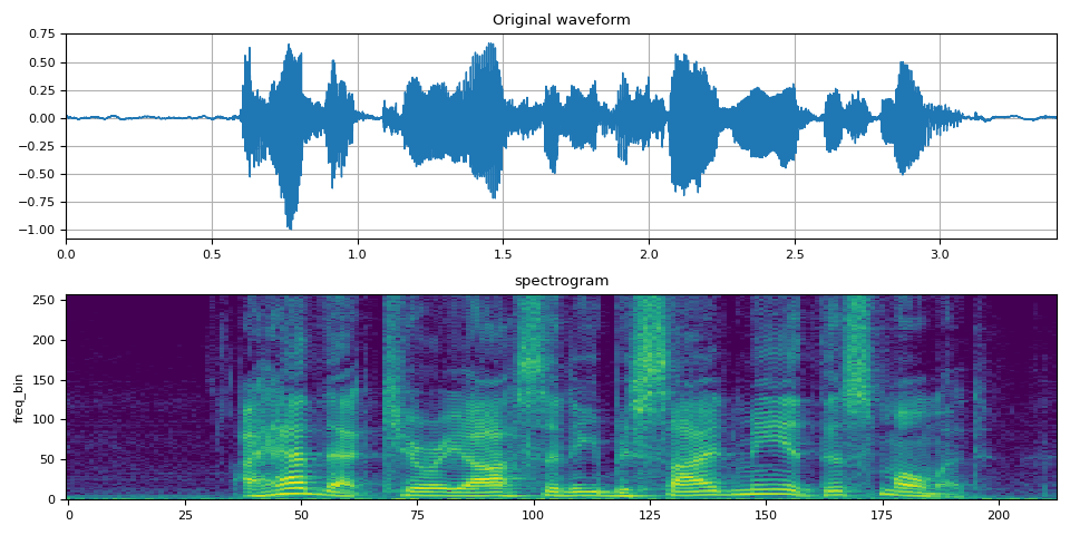
Spectrogram

To get the frequency make-up of an audio signal as it varies with time, you can use torchaudio.transforms.Spectrogram().

# Load audio
SPEECH_WAVEFORM, SAMPLE_RATE = torchaudio.load(SAMPLE_SPEECH)

# Define transform
spectrogram = T.Spectrogram(n_fft=512)

# Perform transform
spec = spectrogram(SPEECH_WAVEFORM)

fig, axs = plt.subplots(2, 1)
plot_waveform(SPEECH_WAVEFORM, SAMPLE_RATE, title="Original waveform", ax=axs[0])
plot_spectrogram(spec[0], title="spectrogram", ax=axs[1])
fig.tight_layout()

Audio(SPEECH_WAVEFORM.numpy(), rate=SAMPLE_RATE)

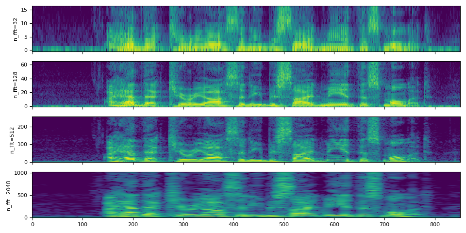
The effect of n_fft parameter

The core of spectrogram computation is (short-term) Fourier transform, and the n_fft parameter corresponds to the \(N\) in the following definition of descrete Fourier transform.

$$ X_k = \sum_{n=0}^{N-1} x_n e^{-\frac{2\pi i}{N} nk} $$

(For the detail of Fourier transform, please refer to Wikipedia.

The value of n_fft determines the resolution of frequency axis. However, with the higher n_fft value, the energy will be distributed among more bins, so when you visualize it, it might look more blurry, even thought they are higher resolution.

The following illustrates this;

Note

hop_length determines the time axis resolution. By default, (i.e. hop_length=None and win_length=None), the value of n_fft // 4 is used. Here we use the same hop_length value across different n_fft so that they have the same number of elemets in the time axis.

n_ffts = [32, 128, 512, 2048]
hop_length = 64

specs = []
for n_fft in n_ffts:
    spectrogram = T.Spectrogram(n_fft=n_fft, hop_length=hop_length)
    spec = spectrogram(SPEECH_WAVEFORM)
    specs.append(spec)

fig, axs = plt.subplots(len(specs), 1, sharex=True)
for i, (spec, n_fft) in enumerate(zip(specs, n_ffts)):
    plot_spectrogram(spec[0], ylabel=f"n_fft={n_fft}", ax=axs[i])
    axs[i].set_xlabel(None)
fig.tight_layout()

When comparing signals, it is desirable to use the same sampling rate, however if you must use the different sampling rate, care must be taken for interpretating the meaning of n_fft. Recall that n_fft determines the resolution of the frequency axis for a given sampling rate. In other words, what each bin on the frequency axis represents is subject to the sampling rate.

As we have seen above, changing the value of n_fft does not change the coverage of frequency range for the same input signal.

Let’s downsample the audio and apply spectrogram with the same n_fft value.

# Downsample to half of the original sample rate
speech2 = torchaudio.functional.resample(SPEECH_WAVEFORM, SAMPLE_RATE, SAMPLE_RATE // 2)
# Upsample to the original sample rate
speech3 = torchaudio.functional.resample(speech2, SAMPLE_RATE // 2, SAMPLE_RATE)

# Apply the same spectrogram
spectrogram = T.Spectrogram(n_fft=512)

spec0 = spectrogram(SPEECH_WAVEFORM)
spec2 = spectrogram(speech2)
spec3 = spectrogram(speech3)

# Visualize it
fig, axs = plt.subplots(3, 1)
plot_spectrogram(spec0[0], ylabel="Original", ax=axs[0])
axs[0].add_patch(Rectangle((0, 3), 212, 128, edgecolor="r", facecolor="none"))
plot_spectrogram(spec2[0], ylabel="Downsampled", ax=axs[1])
plot_spectrogram(spec3[0], ylabel="Upsampled", ax=axs[2])
fig.tight_layout()

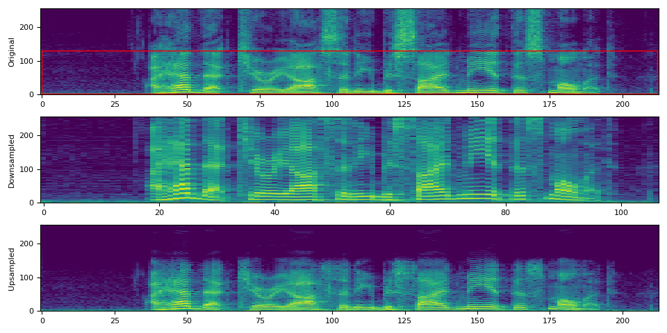
In the above visualization, the second plot (“Downsampled”) might give the impression that the spectrogram is streched. This is because the meaning of frequency bins is different from the original one. Even though, they have the same number of bins, in the second plot, the frequency is only covered to the half of the original sampling rate. This becomes more clear if we resample the downsampled signal again so that it has the same sample rate as the original.

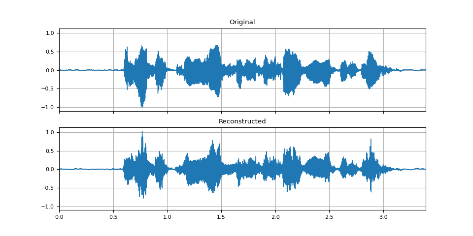
GriffinLim

To recover a waveform from a spectrogram, you can use torchaudio.transforms.GriffinLim.

The same set of parameters used for spectrogram must be used.

# Define transforms
n_fft = 1024
spectrogram = T.Spectrogram(n_fft=n_fft)
griffin_lim = T.GriffinLim(n_fft=n_fft)

# Apply the transforms
spec = spectrogram(SPEECH_WAVEFORM)
reconstructed_waveform = griffin_lim(spec)

_, axes = plt.subplots(2, 1, sharex=True, sharey=True)
plot_waveform(SPEECH_WAVEFORM, SAMPLE_RATE, title="Original", ax=axes[0])
plot_waveform(reconstructed_waveform, SAMPLE_RATE, title="Reconstructed", ax=axes[1])
Audio(reconstructed_waveform, rate=SAMPLE_RATE)

Mel Filter Bank

torchaudio.functional.melscale_fbanks() generates the filter bank for converting frequency bins to mel-scale bins.

Since this function does not require input audio/features, there is no equivalent transform in torchaudio.transforms().

n_fft = 256
n_mels = 64
sample_rate = 6000

mel_filters = F.melscale_fbanks(
    int(n_fft // 2 + 1),
    n_mels=n_mels,
    f_min=0.0,
    f_max=sample_rate / 2.0,
    sample_rate=sample_rate,
    norm="slaney",
)

plot_fbank(mel_filters, "Mel Filter Bank - torchaudio")

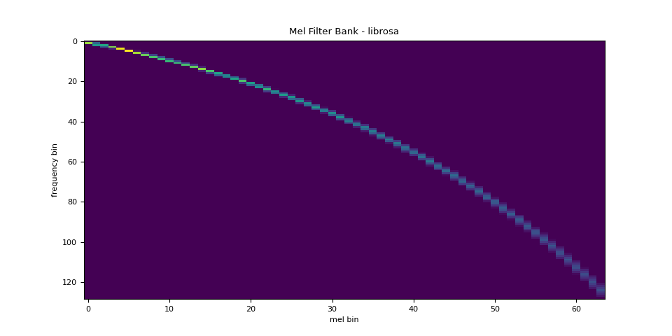
Comparison against librosa

For reference, here is the equivalent way to get the mel filter bank with librosa.

mel_filters_librosa = librosa.filters.mel(
    sr=sample_rate,
    n_fft=n_fft,
    n_mels=n_mels,
    fmin=0.0,
    fmax=sample_rate / 2.0,
    norm="slaney",
    htk=True,
).T

plot_fbank(mel_filters_librosa, "Mel Filter Bank - librosa")

mse = torch.square(mel_filters - mel_filters_librosa).mean().item()
print("Mean Square Difference: ", mse)

Mean Square Difference:  3.934872696751886e-17

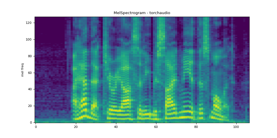
MelSpectrogram

Generating a mel-scale spectrogram involves generating a spectrogram and performing mel-scale conversion. In torchaudio, torchaudio.transforms.MelSpectrogram() provides this functionality.

n_fft = 1024
win_length = None
hop_length = 512
n_mels = 128

mel_spectrogram = T.MelSpectrogram(
    sample_rate=sample_rate,
    n_fft=n_fft,
    win_length=win_length,
    hop_length=hop_length,
    center=True,
    pad_mode="reflect",
    power=2.0,
    norm="slaney",
    n_mels=n_mels,
    mel_scale="htk",
)

melspec = mel_spectrogram(SPEECH_WAVEFORM)

plot_spectrogram(melspec[0], title="MelSpectrogram - torchaudio", ylabel="mel freq")

Comparison against librosa

For reference, here is the equivalent means of generating mel-scale spectrograms with librosa.

melspec_librosa = librosa.feature.melspectrogram(
    y=SPEECH_WAVEFORM.numpy()[0],
    sr=sample_rate,
    n_fft=n_fft,
    hop_length=hop_length,
    win_length=win_length,
    center=True,
    pad_mode="reflect",
    power=2.0,
    n_mels=n_mels,
    norm="slaney",
    htk=True,
)

plot_spectrogram(melspec_librosa, title="MelSpectrogram - librosa", ylabel="mel freq")

mse = torch.square(melspec - melspec_librosa).mean().item()
print("Mean Square Difference: ", mse)

Mean Square Difference:  1.2895221557229775e-09

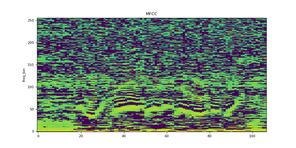
MFCC

n_fft = 2048
win_length = None
hop_length = 512
n_mels = 256
n_mfcc = 256

mfcc_transform = T.MFCC(
    sample_rate=sample_rate,
    n_mfcc=n_mfcc,
    melkwargs={
        "n_fft": n_fft,
        "n_mels": n_mels,
        "hop_length": hop_length,
        "mel_scale": "htk",
    },
)

mfcc = mfcc_transform(SPEECH_WAVEFORM)

plot_spectrogram(mfcc[0], title="MFCC")

Comparison against librosa

melspec = librosa.feature.melspectrogram(
    y=SPEECH_WAVEFORM.numpy()[0],
    sr=sample_rate,
    n_fft=n_fft,
    win_length=win_length,
    hop_length=hop_length,
    n_mels=n_mels,
    htk=True,
    norm=None,
)

mfcc_librosa = librosa.feature.mfcc(
    S=librosa.core.spectrum.power_to_db(melspec),
    n_mfcc=n_mfcc,
    dct_type=2,
    norm="ortho",
)

plot_spectrogram(mfcc_librosa, title="MFCC (librosa)")

mse = torch.square(mfcc - mfcc_librosa).mean().item()
print("Mean Square Difference: ", mse)

Mean Square Difference:  0.8104011416435242

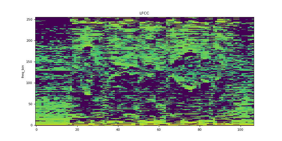
LFCC

n_fft = 2048
win_length = None
hop_length = 512
n_lfcc = 256

lfcc_transform = T.LFCC(
    sample_rate=sample_rate,
    n_lfcc=n_lfcc,
    speckwargs={
        "n_fft": n_fft,
        "win_length": win_length,
        "hop_length": hop_length,
    },
)

lfcc = lfcc_transform(SPEECH_WAVEFORM)
plot_spectrogram(lfcc[0], title="LFCC")

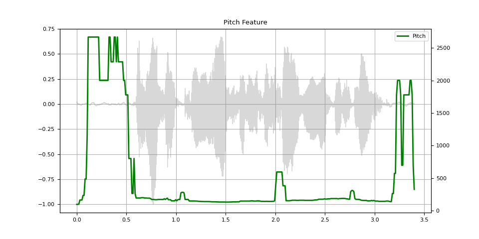
Pitch

pitch = F.detect_pitch_frequency(SPEECH_WAVEFORM, SAMPLE_RATE)

def plot_pitch(waveform, sr, pitch):
    figure, axis = plt.subplots(1, 1)
    axis.set_title("Pitch Feature")
    axis.grid(True)

    end_time = waveform.shape[1] / sr
    time_axis = torch.linspace(0, end_time, waveform.shape[1])
    axis.plot(time_axis, waveform[0], linewidth=1, color="gray", alpha=0.3)

    axis2 = axis.twinx()
    time_axis = torch.linspace(0, end_time, pitch.shape[1])
    axis2.plot(time_axis, pitch[0], linewidth=2, label="Pitch", color="green")

    axis2.legend(loc=0)


plot_pitch(SPEECH_WAVEFORM, SAMPLE_RATE, pitch)