Pytorch/XLA overview
This section provides a brief overview of the basic details of PyTorch XLA, which should help readers better understand the required modifications and optimizations of code.
Unlike regular PyTorch, which executes code line by line and does not block execution until the value of a PyTorch tensor is fetched, PyTorch XLA works differently. It iterates through the python code and records the operations on (PyTorch) XLA tensors in an intermediate representation (IR) graph until it encounters a barrier (discussed below). This process of generating the IR graph is referred to as tracing (LazyTensor tracing or code tracing). PyTorch XLA then converts the IR graph to a lower-level machine-readable format called HLO (High-Level Opcodes). HLO is a representation of a computation that is specific to the XLA compiler and allows it to generate efficient code for the hardware that it is running on. HLO is fed to the XLA compiler for compilation and optimization. Compilation is then cached by PyTorch XLA to be reused later if/when needed. The compilation of the graph is done on the host (CPU), which is the machine that runs the Python code. If there are multiple XLA devices, the host compiles the code for each of the devices separately except when using SPMD (single-program, multiple-data). For example, v4-8 has one host machine and four devices. In this case the host compiles the code for each of the four devices separately. In case of pod slices, when there are multiple hosts, each host does the compilation for XLA devices it is attached to. If SPMD is used, then the code is compiled only once (for given shapes and computations) on each host for all the devices.

For more details and examples, please refer to the LazyTensor guide.
The operations in the IR graph are executed only when values of tensors are needed. This is referred to as evaluation or materialization of tensors. Sometimes this is also called lazy evaluation and it can lead to significant performance improvements.
The synchronous operations in Pytorch XLA, like printing, logging,
checkpointing or callbacks block tracing and result in slower execution.
In the case when an operation requires a specific value of an XLA
tensor, e.g. print(xla_tensor_z), tracing is blocked until the value
of that tensor is available to the host. Note that only the part of the
graph responsible for computing that tensor value is executed. These
operations do not cut the IR graph, but they trigger host-device
communication through TransferFromDevice, which results in slower
performance.
A barrier is a special instruction that tells XLA to execute the IR
graph and materialize the tensors. This means that the PyTorch XLA
tensors will be evaluated, and the results will be available to the
host. The user-exposed barrier in Pytorch XLA is
xm.mark_step(),
which breaks the IR graph and results in code execution on the XLA
devices. One of the key properties of xm.mark_step is that unlike
synchronous operations it does not block the further tracing while the
device is executing the graph. However, it does block access to the
values of the tensors that are being materialized.
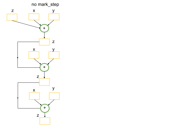
The example in the LazyTensor guide illustrates what happens in a simple case of adding two tensors. Now, suppose we have a for loop that adds XLA tensors and uses the value later:
for x, y in tensors_on_device:
    z += x + y
Without a barrier, the Python tracing will result in a single graph that
wraps the addition of tensors len(tensors_on_device) times. This is
because the for loop is not captured by the tracing, so each iteration
of the loop will create a new subgraph corresponding to the computation
of z += x+y and add it to the graph. Here is an example when
len(tensors_on_device)=3.
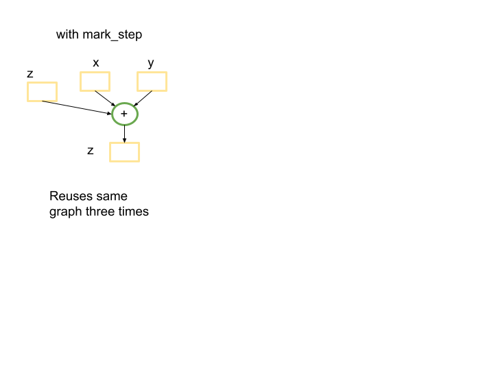
However, introducing a barrier at the end of the loop will result in a
smaller graph that will be compiled once during the first pass inside
the for loop and will be reused for the next
len(tensors_on_device)-1 iterations. The barrier will signal to the
tracing that the graph traced so far can be submitted for execution, and
if that graph has been seen before, a cached compiled program will be
reused.
for x, y in tensors_on_device:
    z += x + y
    xm.mark_step()
In this case there will be a small graph that is used
len(tensors_on_device)=3 times.
It is important to highlight that in PyTorch XLA Python code inside for loops is traced and a new graph is constructed for each iteration if there is a barrier at the end. This can be a significant performance bottleneck.
The XLA graphs can be reused when the same computation happens on the same shapes of tensors. If the shapes of the inputs or intermediate tensors change, then the XLA compiler will recompile a new graph with the new tensor shapes. This means that if you have dynamic shapes or if your code does not reuse tensor graphs, running your model on XLA will not be suitable for that use case. Padding the input into a fixed shape can be an option to help avoid dynamic shapes. Otherwise, a significant amount of time will be spent by the compiler on optimizing and fusing operations which will not be used again.
The trade-off between graph size and compilation time is also important to consider. If there is one large IR graph, the XLA compiler can spend a lot of time on optimization and fusion of the ops. This can result in a very long compilation time. However, the later execution may be much faster, due to the optimizations that were performed during compilation.
Sometimes it is worth breaking the IR graph with xm.mark_step(). As
explained above, this will result in a smaller graph that can be reused
later. However making graphs smaller can reduce optimizations that
otherwise could be done by the XLA compiler.
Another important point to consider is
MPDeviceLoader.
Once your code is running on an XLA device, consider wrapping the torch
dataloader with XLA MPDeviceLoader which preloads data to the device
to improve performance and includes xm.mark_step() in it. The latter
automatically breaks the iterations over batches of data and sends them
for execution. Note, if you are not using MPDeviceLoader, you might need
to set barrier=True in the optimizer_step() to enable
xm.mark_step() if running a training job or explicitly adding
xm.mark_step().
TPU Setup
Create TPU with base image to use nightly wheels or from the stable
release by specifying the RUNTIME_VERSION.
export ZONE=us-central2-b
export PROJECT_ID=your-project-id
export ACCELERATOR_TYPE=v4-8 # v4-16, v4-32, …
export RUNTIME_VERSION=tpu-vm-v4-pt-2.0 # or tpu-vm-v4-base
export TPU_NAME=your_tpu_name

gcloud compute tpus tpu-vm create ${TPU_NAME} \
--zone=${ZONE} \
--accelerator-type=${ACCELERATOR_TYPE} \
--version=${RUNTIME_VERSION} \
--subnetwork=tpusubnet
If you have a single host VM (e.g. v4-8), you can ssh to your vm and run
the following commands from the vm directly. Otherwise, in case of TPU
pods, you can use --worker=all --command="" similar to
gcloud compute tpus tpu-vm ssh ${TPU_NAME} \
--zone=us-central2-b \
--worker=all \
--command="pip3 install https://storage.googleapis.com/pytorch-xla-releases/wheels/tpuvm/torch-nightly-cp38-cp38-linux_x86_64.whl"
Next, if you are using base image, install nightly packages and required libraries
pip3 install https://storage.googleapis.com/pytorch-xla-releases/wheels/tpuvm/torch-nightly-cp38-cp38-linux_x86_64.whl
pip3 install https://storage.googleapis.com/pytorch-xla-releases/wheels/tpuvm/torch_xla-nightly-cp38-cp38-linux_x86_64.whl
sudo apt-get install libopenblas-dev -y
sudo apt-get update && sudo apt-get install libgl1 -y # diffusion specific
Reference implementations
The AI-Hypercomputer/tpu-recipies repo. contains examples for training and serving many LLM and diffusion models.
Converting code to PyTorch XLA
General guidelines to modify your code:
Replace
cudawithxm.xla_device()Remove progress bar, printing that would access the XLA tensor values
Reduce logging and callbacks that would access the XLA tensor values
Wrap data loader with MPDeviceLoader
Profile to further optimize the code
Remember: each case is unique so you might need to do something different for each case.
Example 1. Stable Diffusion inference in PyTorch Lightning on a Single TPU Device
As a first example consider the inference code of the stable diffusion model in PyTorch Lightning which can be run from command line as
python scripts/txt2img.py --prompt "a photograph of an astronaut riding a horse"
For your reference, the diff of modifications described below can be
found
here.
Let’s go over them step by step. As in the general guideline above,
start with changes related to cuda device. This inference code is
written to run on GPUs and cuda can be found in multiple places. Start
making changes by removing model.cuda() from this
line,
and precision_scope from
here.
Additionally, replace the cuda device in this
line
with the xla device similar to the code below:
Next, this particular configuration of the model is using
FrozenCLIPEmbedder, therefore we will modify this
line
as well. For simplicity we will directly define the device in this
tutorial, but you can pass the device value to the function as well.
import torch_xla.core.xla_model as xm
self.device = xm.xla_device()
Another place in the code that has cuda specific code is DDIM scheduler.
Add import torch_xla.core.xla_model as xm on top of the file then
replace
these
lines
if attr.device != torch.device("cuda"):
   attr = attr.to(torch.device("cuda"))
with
device = xm.xla_device()
attr = attr.to(torch.device(device))
Next, you can reduce device (TPU) and host (CPU) communication by removing print statements, disabling progress bars, and reducing or removing callbacks and logging. These operations require the device to stop executing, falling back to the CPU, executing the logging/callbacks, and then returning to the device. This can be a significant performance bottleneck, especially on large models.
After making these changes, the code will run on TPUs. However, the performance will be very slow. This is because the XLA compiler tries to build a single (huge) graph that wraps the number of inference steps (in this case, 50) as there is no barrier inside the for loop. It is difficult for the compiler to optimize the graph, and this leads to significant performance degradation. As discussed above, breaking the for loop with the barrier (xm.mark_step()) will result in a smaller graph that is easier for the compiler to optimize. This will also allow the compiler to reuse the graph from the previous step, which can improve performance.
Now the code is ready to run on TPUs in a reasonable time. More optimization and analysis can be done by capturing a profile and investigating further. However, this is not covered here.
Note: if you are running on v4-8 TPU, then you have 4 available XLA
(TPU) devices. Running the code as above will only use one XLA device.
In order to run on all 4 devices you need to use torch_xla.launch()
function to spawn the code on all the devices. We will discuss a
torch_xla.launch in the next example.
Example 2. HF Stable Diffusion Inference
Now, consider using Stable Diffusion Inference in the HuggingFace diffusers library for both the SD-XL and 2.1 versions of the model. For your reference, the changes described below can be found in this repo. You can clone the repo and run the inference using the following command on your TPU VM:
(vm)$ git clone https://github.com/pytorch-tpu/diffusers.git
(vm)$ cd diffusers/examples/text_to_image/
(vm)$ python3 inference_tpu_single_device.py
Running on a Single TPU device
This section describes the changes that need to be made to the text_to_image inference example code to run it on TPUs.
The original code uses Lora for inference, but this tutorial will not
use it. Instead, we will set the model_id argument to
stabilityai/stable-diffusion-xl-base-0.9 when initializing the
pipeline. We will also use the default scheduler
(DPMSolverMultistepScheduler). However, similar changes can be made to
the other schedulers as well.
git clone https://github.com/huggingface/diffusers
cd diffusers
pip install . # pip install -e .

cd examples/text_to_image/
pip install -r requirements.txt
pip install invisible_watermark transformers accelerate safetensors
(If accelerate is not found, log out, log back in.)
Log in to HF and agree to the sd-xl 0.9 license on the model card. Next, go to account→settings→access token and generate a new token. Copy the token and run the following command with that specific token value on your vm
(vm)$ huggingface-cli login --token _your_copied_token__
The HuggingFace readme provides PyTorch code that is written to run on
GPUs. To run it on TPUs, the first step is to change the CUDA device to
an XLA device. This can be done by replacing the line pipe.to("cuda")
with the following lines:
import torch_xla.core.xla_model as xm
device = xm.xla_device()
pipe.to(device)
Additionally, it is important to note that the first time you run inference with XLA, it will take a long time to compile. For example, compilation time for stable diffusion XL model inference from HuggingFace can take about an hour to compile, whereas the actual inference may take only 5 seconds, depending on the batch size. Likewise, a GPT-2 model can take about 10-15 mins to compile, after which the training epoch time becomes much faster. This is because XLA builds a graph of the computation that will be performed, and then optimizes this graph for the specific hardware that it is running on. However, once the graph has been compiled, it can be reused for subsequent inferences, which will be much faster. Therefore, if you are only running inference once, you may not benefit from using XLA. However, if you are running inference multiple times, or if you are running inference on a list of prompts, you will start to see the advantages of XLA after the first few inferences. For example, if you run inference on a list of 10 prompts, the first inference (maybe two[^1]) may take a long time to compile, but the remaining inference steps will be much faster. This is because XLA will reuse the graph that it compiled for the first inference.
If you try to run the code without making any additional changes, you
will notice that the compilation time is very long (>6 hours). This is
because the XLA compiler tries to build a single graph for all of the
scheduler steps at once similar to what we have discussed in the
previous example. To make the code run faster, we need to break the
graph up into smaller pieces with xm.mark_step() and reuse them in the
next steps. This happens inside the pipe.__call__
function
in these
lines.
Disabling the progress bar, removing callbacks and adding
xm.mark_step() at the end of the for loop speeds up the code
significantly. Changes are provided in this
commit.
Additionally, the self.scheduler.step() function, which by default
uses the DPMSolverMultistepScheduler scheduler, has a few issues that
are described in the PyTorch XLA
caveats.
The .nonzero() and .item() calls in this function send requests to
the CPU for tensor evaluation, which trigger device-host communication.
This is not desirable, as it can slow down the code. In this particular
case, we can avoid these calls by passing the index to the function
directly. This will prevent the function from sending requests to the
CPU, and will improve the performance of the code. Changes are available
in
this
commit. The code now is ready to be run on TPUs.
Profiling and performance analysis
To further investigate the performance of the model, we can profile it using the profiling guide. As a rule of thumb, the profiling script should be run with the maximum batch size that fits into the memory for optimal memory usage. It also helps to overlap tracing of the code with device execution which leads to more optimal device usage. The duration of profiling should be long enough to capture at least one step. Good performance of the model on TPUs means that device-host communication is minimized and the device is constantly running processes with no idle time.
Starting a server in the inference_tpu_*.py file and running
capture_profile.py script as described in the guide will give us
information on processes that run on the devices. Currently, only one
XLA device is profiled. To better understand the TPU idle time (gaps in
the profile), profiling traces (xp.Trace()) should be added to the
code. The xp.Trace() measures the time it takes to trace the python
code on the host machine wrapped with the trace. For this example,
xp.Trace() traces were added inside the
pipeline
and the U-net
model
to measure the time to run specific sections of the code on the host
(CPU).
If the gaps in the profile are due to Python code tracing that happens
on the host, then this might be a bottleneck and there is no further
straightforward optimization that can be done. Otherwise, the code
should be analyzed further to understand the caveats and improve the
performance further. Note that you cannot xp.Trace() wrap portions of
the code where xm.mark_step() is called.
To illustrate this we can look at already captured profiles that were uploaded to tensorboard following the profiling guide.
Starting from Stable Diffusion model version 2.1
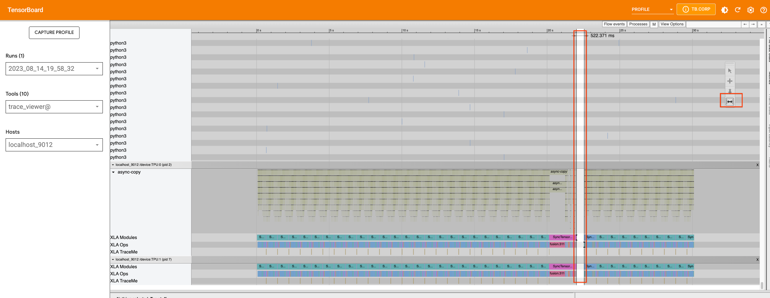
If we capture a profile without inserting any traces, we will see the following:
The single TPU device on v4-8, which has two cores, appears to be busy.
There are no significant gaps in their usage, except for a small one in
the middle. If we scroll up to try to find which process is occupying
the host machine, we will not find any information. Therefore, we will
add xp.traces to the pipeline
file
as well as the U-net
function.
The latter may not be useful for this particular use case, but it does
demonstrate how traces can be added in different places and how their
information is displayed in TensorBoard.
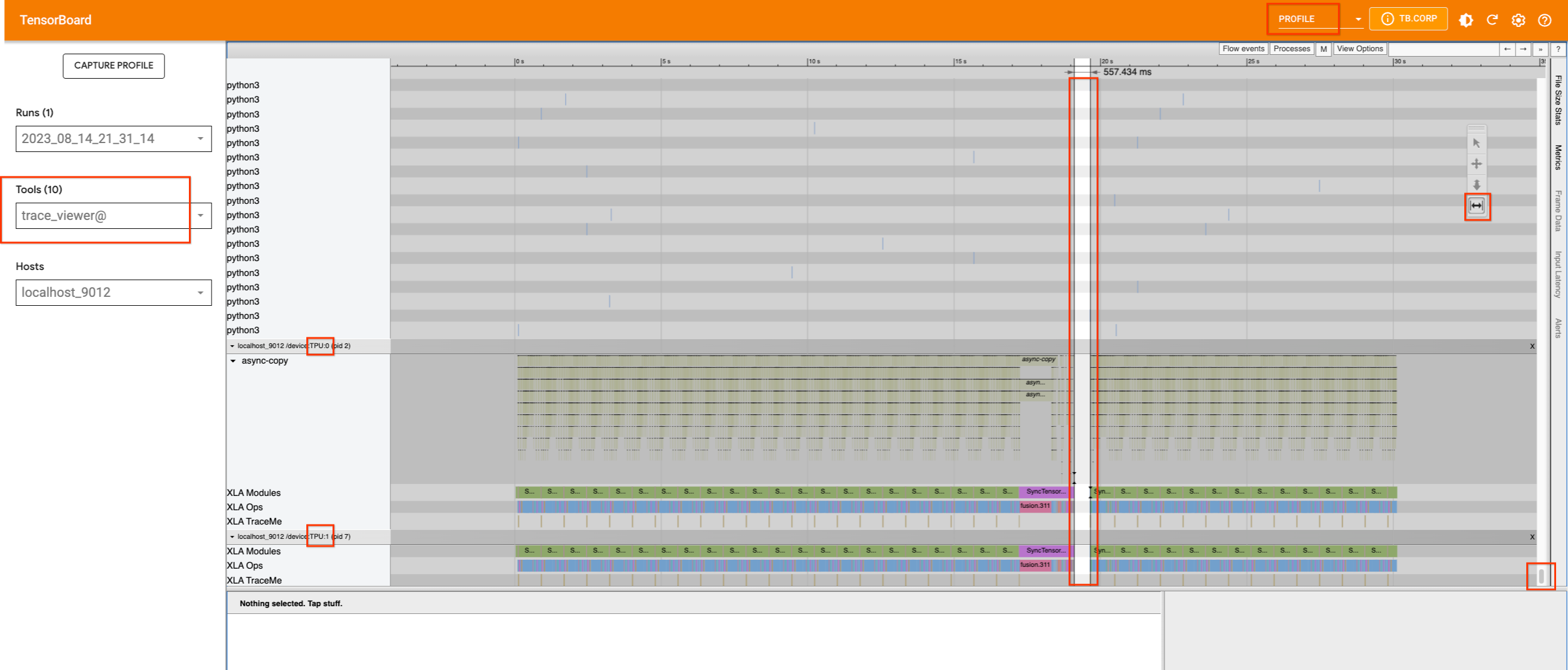
If we add traces and re-capture the profile with the largest batch size that can fit on the device (32 in this case), we will see that the gap in the device is caused by a Python process that is running on the host machine.
We can use the appropriate tool to zoom in on the timeline and see which process is running during that period. This is when the Python code tracing happens on the host, and we cannot improve the tracing further at this point.
Now, let’s examine the XL version of the model and do the same thing. We will add traces to the pipeline file in the same way that we did for the 2.1 version and capture a profile.
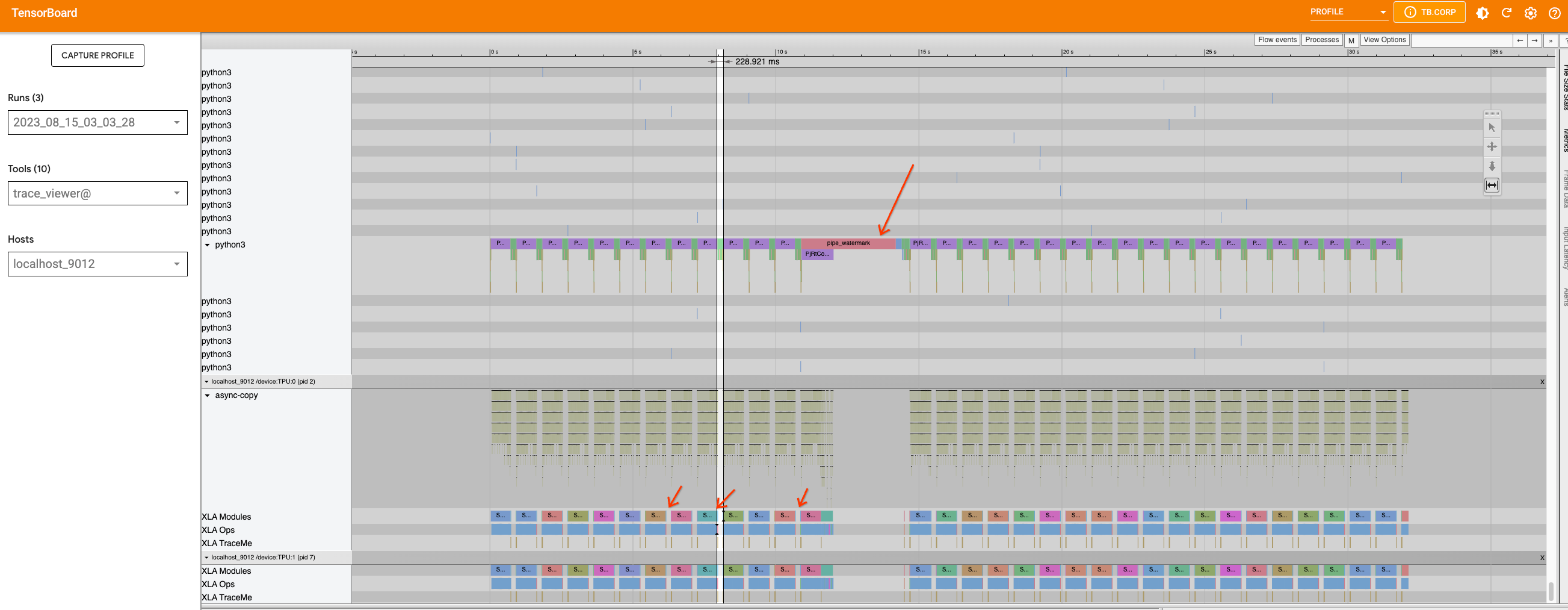
This time, in addition to the large gap in the middle, which is caused
by the pipe_watermark tracing, there are many small gaps between the
inference steps within this
loop.
First look closer into the large gap that is caused by pipe_watermark.
The gap is preceded with TransferFromDevice which indicates that
something is happening on the host machine that is waiting for
computation to finish before proceeding. Looking into watermark
code,
we can see that tensors are transferred to cpu and converted to numpy
arrays in order to be processed with cv2 and pywt libraries later.
Since this part is not straightforward to optimize, we will leave this
as is.
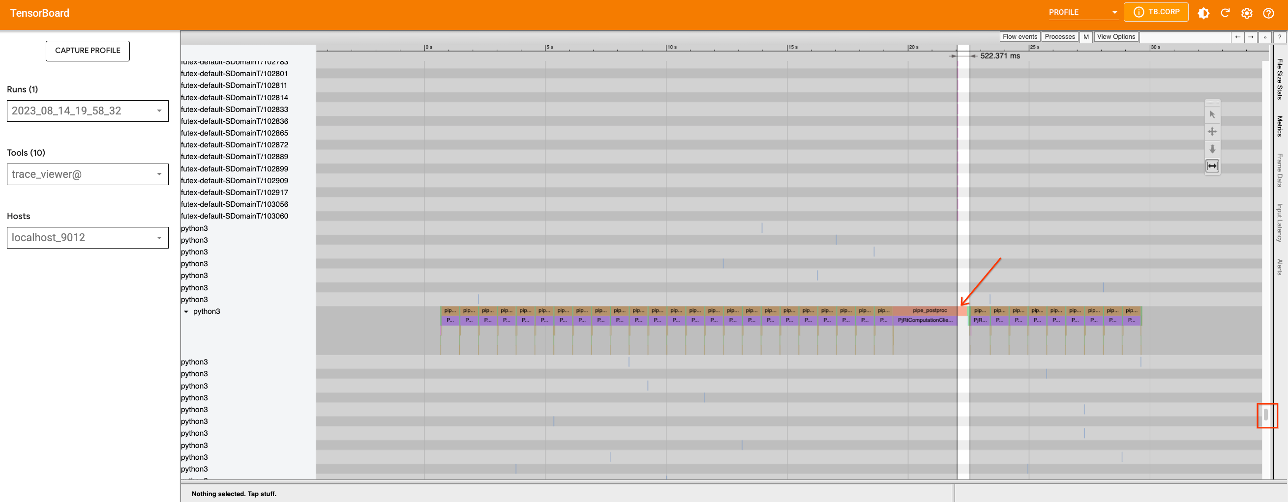
Now if we zoom in on the loop, we can see that the graph within the loop
is broken into smaller parts because the TransferFromDevice operation
happens.
If we investigate the U-Net function and the scheduler, we can see that
the U-Net code does not contain any optimization targets for
PyTorch/XLA. However, there are .item() and .nonzero() calls inside
the
scheduler.step.
We can
rewrite
the function to avoid those calls. If we fix this issue and rerun a
profile, we will not see much difference. However, since we have reduced
the device-host communication that was introducing smaller graphs, we
allowed the compiler to optimize the code better. The function
scale_model_input
has similar issues, and we can fix these by making the changes we made
above to the step function. Overall, since many of the gaps are caused
from python level code tracing and graph building, these gaps are not
possible to optimize with the current version of PyTorch XLA, but we may
see improvements in the future when dynamo is enabled in PyTorch XLA.
Running on Multiple TPU Devices
To use multiple TPU devices, you can use the torch_xla.launch function
to spawn the function you ran on a single device to multiple devices.
The torch_xla.launch function will start processes on multiple TPU
devices and sync them when needed. This can be done by passing the
index argument to the function that runs on a single device. For
example,
import torch_xla

def my_function(index):
  # function that runs on a single device

torch_xla.launch(my_function, args=(0,))
In this example, the my_function function will be spawned on 4 TPU
devices on v4-8, with each device being assigned an index from 0 to 3.
Note that by default, the launch() function will spawn preocesses on all
TPU devices. If you only want to run single process, set the argument
launch(..., debug_single_process=True).
This file illustrates how xmp.spawn can be used to run stable diffusion 2.1 version on multiple TPU devices. For this version similar to the above changes were made to the pipeline file.
Running on Pods
Once you have the code for running on a single host device, there is no further change needed. You can create the TPU pod, for example, by following these instructions. Then run your script with
gcloud compute tpus tpu-vm ssh ${TPU_NAME} \
  --zone=${ZONE} \
  --worker=all \
  --command="python3 your_script.py"
Note:
0 and 1 are magic numbers in XLA and treated as constants in the
HLO. So if there is a random number generator in the code that can
generate these values, the code will compile for each value
separately. This can be disabled with XLA_NO_SPECIAL_SCALARS=1
environment variable.
