Torchaudio-Squim: Non-intrusive Speech Assessment in TorchAudio

Author: Anurag Kumar, Zhaoheng Ni

1. Overview

This tutorial shows uses of Torchaudio-Squim to estimate objective and subjective metrics for assessment of speech quality and intelligibility.

TorchAudio-Squim enables speech assessment in Torchaudio. It provides interface and pre-trained models to estimate various speech quality and intelligibility metrics. Currently, Torchaudio-Squim [1] supports reference-free estimation 3 widely used objective metrics:

• Wideband Perceptual Estimation of Speech Quality (PESQ) [2]

• Short-Time Objective Intelligibility (STOI) [3]

• Scale-Invariant Signal-to-Distortion Ratio (SI-SDR) [4]

It also supports estimation of subjective Mean Opinion Score (MOS) for a given audio waveform using Non-Matching References [1, 5].

References

[1] Kumar, Anurag, et al. “TorchAudio-Squim: Reference-less Speech Quality and Intelligibility measures in TorchAudio.” ICASSP 2023-2023 IEEE International Conference on Acoustics, Speech and Signal Processing (ICASSP). IEEE, 2023.

[2] I. Rec, “P.862.2: Wideband extension to recommendation P.862 for the assessment of wideband telephone networks and speech codecs,” International Telecommunication Union, CH–Geneva, 2005.

[3] Taal, C. H., Hendriks, R. C., Heusdens, R., & Jensen, J. (2010, March). A short-time objective intelligibility measure for time-frequency weighted noisy speech. In 2010 IEEE international conference on acoustics, speech and signal processing (pp. 4214-4217). IEEE.

[4] Le Roux, Jonathan, et al. “SDR–half-baked or well done?.” ICASSP 2019-2019 IEEE International Conference on Acoustics, Speech and Signal Processing (ICASSP). IEEE, 2019.

[5] Manocha, Pranay, and Anurag Kumar. “Speech quality assessment through MOS using non-matching references.” Interspeech, 2022.

import torch
import torchaudio

print(torch.__version__)
print(torchaudio.__version__)

2.4.0.dev20240416
2.2.0.dev20240418

2. Preparation

First import the modules and define the helper functions.

We will need torch, torchaudio to use Torchaudio-squim, Matplotlib to plot data, pystoi, pesq for computing reference metrics.

try:
    from pesq import pesq
    from pystoi import stoi
    from torchaudio.pipelines import SQUIM_OBJECTIVE, SQUIM_SUBJECTIVE
except ImportError:
    try:
        import google.colab  # noqa: F401

        print(
            """
            To enable running this notebook in Google Colab, install nightly
            torch and torchaudio builds by adding the following code block to the top
            of the notebook before running it:
            !pip3 uninstall -y torch torchvision torchaudio
            !pip3 install --pre torch torchvision torchaudio --extra-index-url https://download.pytorch.org/whl/nightly/cpu
            !pip3 install pesq
            !pip3 install pystoi
            """
        )
    except Exception:
        pass
    raise


import matplotlib.pyplot as plt

import torchaudio.functional as F
from IPython.display import Audio
from torchaudio.utils import download_asset


def si_snr(estimate, reference, epsilon=1e-8):
    estimate = estimate - estimate.mean()
    reference = reference - reference.mean()
    reference_pow = reference.pow(2).mean(axis=1, keepdim=True)
    mix_pow = (estimate * reference).mean(axis=1, keepdim=True)
    scale = mix_pow / (reference_pow + epsilon)

    reference = scale * reference
    error = estimate - reference

    reference_pow = reference.pow(2)
    error_pow = error.pow(2)

    reference_pow = reference_pow.mean(axis=1)
    error_pow = error_pow.mean(axis=1)

    si_snr = 10 * torch.log10(reference_pow) - 10 * torch.log10(error_pow)
    return si_snr.item()


def plot(waveform, title, sample_rate=16000):
    wav_numpy = waveform.numpy()

    sample_size = waveform.shape[1]
    time_axis = torch.arange(0, sample_size) / sample_rate

    figure, axes = plt.subplots(2, 1)
    axes[0].plot(time_axis, wav_numpy[0], linewidth=1)
    axes[0].grid(True)
    axes[1].specgram(wav_numpy[0], Fs=sample_rate)
    figure.suptitle(title)

3. Load Speech and Noise Sample

SAMPLE_SPEECH = download_asset("tutorial-assets/Lab41-SRI-VOiCES-src-sp0307-ch127535-sg0042.wav")
SAMPLE_NOISE = download_asset("tutorial-assets/Lab41-SRI-VOiCES-rm1-babb-mc01-stu-clo.wav")

  0%|          | 0.00/156k [00:00<?, ?B/s]
100%|##########| 156k/156k [00:00<00:00, 92.1MB/s]

WAVEFORM_SPEECH, SAMPLE_RATE_SPEECH = torchaudio.load(SAMPLE_SPEECH)
WAVEFORM_NOISE, SAMPLE_RATE_NOISE = torchaudio.load(SAMPLE_NOISE)
WAVEFORM_NOISE = WAVEFORM_NOISE[0:1, :]

Currently, Torchaudio-Squim model only supports 16000 Hz sampling rate. Resample the waveforms if necessary.

if SAMPLE_RATE_SPEECH != 16000:
    WAVEFORM_SPEECH = F.resample(WAVEFORM_SPEECH, SAMPLE_RATE_SPEECH, 16000)

if SAMPLE_RATE_NOISE != 16000:
    WAVEFORM_NOISE = F.resample(WAVEFORM_NOISE, SAMPLE_RATE_NOISE, 16000)

Trim waveforms so that they have the same number of frames.

if WAVEFORM_SPEECH.shape[1] < WAVEFORM_NOISE.shape[1]:
    WAVEFORM_NOISE = WAVEFORM_NOISE[:, : WAVEFORM_SPEECH.shape[1]]
else:
    WAVEFORM_SPEECH = WAVEFORM_SPEECH[:, : WAVEFORM_NOISE.shape[1]]

Play speech sample

Audio(WAVEFORM_SPEECH.numpy()[0], rate=16000)

Play noise sample

Audio(WAVEFORM_NOISE.numpy()[0], rate=16000)

4. Create distorted (noisy) speech samples

snr_dbs = torch.tensor([20, -5])
WAVEFORM_DISTORTED = F.add_noise(WAVEFORM_SPEECH, WAVEFORM_NOISE, snr_dbs)

Play distorted speech with 20dB SNR

Audio(WAVEFORM_DISTORTED.numpy()[0], rate=16000)

Play distorted speech with -5dB SNR

Audio(WAVEFORM_DISTORTED.numpy()[1], rate=16000)

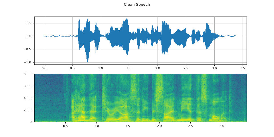
5. Visualize the waveforms

Visualize speech sample

plot(WAVEFORM_SPEECH, "Clean Speech")

Visualize noise sample

plot(WAVEFORM_NOISE, "Noise")

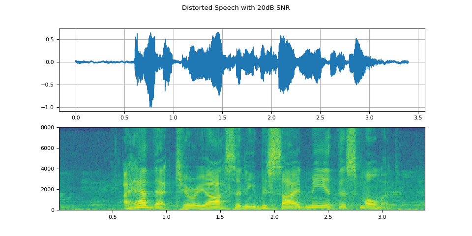
Visualize distorted speech with 20dB SNR

plot(WAVEFORM_DISTORTED[0:1], f"Distorted Speech with {snr_dbs[0]}dB SNR")

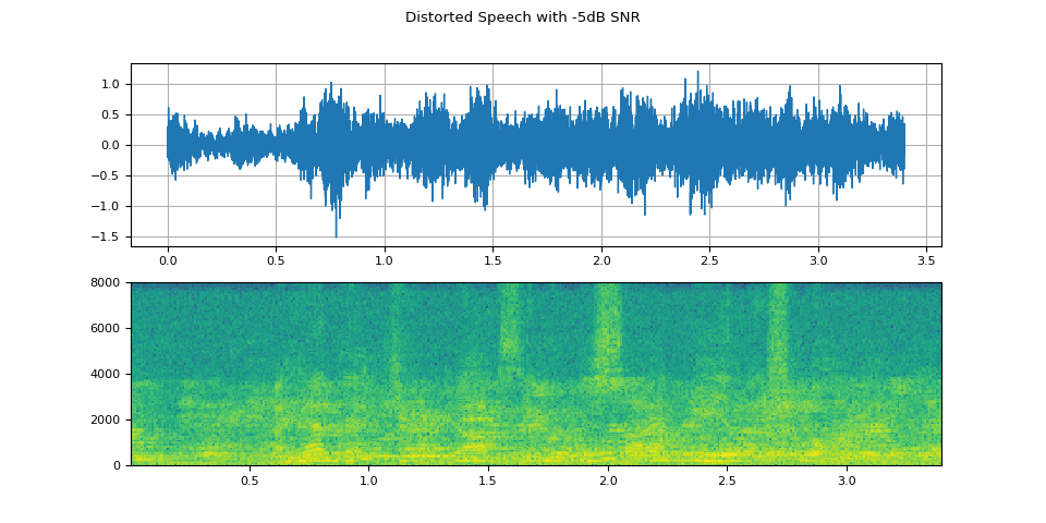
Visualize distorted speech with -5dB SNR

plot(WAVEFORM_DISTORTED[1:2], f"Distorted Speech with {snr_dbs[1]}dB SNR")

6. Predict Objective Metrics

Get the pre-trained SquimObjectivemodel.

objective_model = SQUIM_OBJECTIVE.get_model()

Downloading: "https://download.pytorch.org/torchaudio/models/squim_objective_dns2020.pth" to /root/.cache/torch/hub/checkpoints/squim_objective_dns2020.pth

  0%|          | 0.00/28.2M [00:00<?, ?B/s]
100%|##########| 28.2M/28.2M [00:00<00:00, 388MB/s]

Compare model outputs with ground truths for distorted speech with 20dB SNR

stoi_hyp, pesq_hyp, si_sdr_hyp = objective_model(WAVEFORM_DISTORTED[0:1, :])
print(f"Estimated metrics for distorted speech at {snr_dbs[0]}dB are\n")
print(f"STOI: {stoi_hyp[0]}")
print(f"PESQ: {pesq_hyp[0]}")
print(f"SI-SDR: {si_sdr_hyp[0]}\n")

pesq_ref = pesq(16000, WAVEFORM_SPEECH[0].numpy(), WAVEFORM_DISTORTED[0].numpy(), mode="wb")
stoi_ref = stoi(WAVEFORM_SPEECH[0].numpy(), WAVEFORM_DISTORTED[0].numpy(), 16000, extended=False)
si_sdr_ref = si_snr(WAVEFORM_DISTORTED[0:1], WAVEFORM_SPEECH)
print(f"Reference metrics for distorted speech at {snr_dbs[0]}dB are\n")
print(f"STOI: {stoi_ref}")
print(f"PESQ: {pesq_ref}")
print(f"SI-SDR: {si_sdr_ref}")

Estimated metrics for distorted speech at 20dB are

STOI: 0.9610356092453003
PESQ: 2.7801527976989746
SI-SDR: 20.692630767822266

Reference metrics for distorted speech at 20dB are

STOI: 0.9670831113894452
PESQ: 2.7961528301239014
SI-SDR: 19.998966217041016

Compare model outputs with ground truths for distorted speech with -5dB SNR

stoi_hyp, pesq_hyp, si_sdr_hyp = objective_model(WAVEFORM_DISTORTED[1:2, :])
print(f"Estimated metrics for distorted speech at {snr_dbs[1]}dB are\n")
print(f"STOI: {stoi_hyp[0]}")
print(f"PESQ: {pesq_hyp[0]}")
print(f"SI-SDR: {si_sdr_hyp[0]}\n")

pesq_ref = pesq(16000, WAVEFORM_SPEECH[0].numpy(), WAVEFORM_DISTORTED[1].numpy(), mode="wb")
stoi_ref = stoi(WAVEFORM_SPEECH[0].numpy(), WAVEFORM_DISTORTED[1].numpy(), 16000, extended=False)
si_sdr_ref = si_snr(WAVEFORM_DISTORTED[1:2], WAVEFORM_SPEECH)
print(f"Reference metrics for distorted speech at {snr_dbs[1]}dB are\n")
print(f"STOI: {stoi_ref}")
print(f"PESQ: {pesq_ref}")
print(f"SI-SDR: {si_sdr_ref}")

Estimated metrics for distorted speech at -5dB are

STOI: 0.5743248462677002
PESQ: 1.1112866401672363
SI-SDR: -6.248741626739502

Reference metrics for distorted speech at -5dB are

STOI: 0.5848137931588825
PESQ: 1.0803768634796143
SI-SDR: -5.016279220581055

7. Predict Mean Opinion Scores (Subjective) Metric

Get the pre-trained SquimSubjective model.

subjective_model = SQUIM_SUBJECTIVE.get_model()

Downloading: "https://download.pytorch.org/torchaudio/models/squim_subjective_bvcc_daps.pth" to /root/.cache/torch/hub/checkpoints/squim_subjective_bvcc_daps.pth

  0%|          | 0.00/360M [00:00<?, ?B/s]
  2%|1         | 6.38M/360M [00:00<00:05, 62.1MB/s]
  5%|4         | 16.5M/360M [00:00<00:07, 50.7MB/s]
  7%|7         | 26.4M/360M [00:00<00:05, 67.4MB/s]
  9%|9         | 33.6M/360M [00:00<00:08, 39.9MB/s]
 13%|#3        | 47.6M/360M [00:01<00:07, 46.3MB/s]
 15%|#4        | 52.9M/360M [00:01<00:08, 39.2MB/s]
 16%|#5        | 57.2M/360M [00:01<00:08, 38.9MB/s]
 18%|#8        | 65.6M/360M [00:01<00:07, 39.2MB/s]
 21%|##        | 74.0M/360M [00:01<00:06, 45.4MB/s]
 22%|##2       | 80.4M/360M [00:01<00:06, 44.3MB/s]
 24%|##3       | 84.9M/360M [00:02<00:07, 39.8MB/s]
 27%|##7       | 98.4M/360M [00:02<00:05, 49.2MB/s]
 32%|###1      | 114M/360M [00:02<00:03, 66.9MB/s]
 34%|###3      | 121M/360M [00:02<00:04, 59.4MB/s]
 36%|###6      | 131M/360M [00:02<00:04, 54.9MB/s]
 41%|####      | 146M/360M [00:02<00:03, 63.7MB/s]
 42%|####2     | 152M/360M [00:03<00:03, 54.8MB/s]
 45%|####5     | 162M/360M [00:03<00:03, 58.3MB/s]
 47%|####6     | 168M/360M [00:03<00:04, 43.2MB/s]
 50%|####9     | 180M/360M [00:03<00:03, 49.9MB/s]
 51%|#####1    | 185M/360M [00:03<00:04, 45.2MB/s]
 54%|#####4    | 195M/360M [00:04<00:03, 53.3MB/s]
 56%|#####5    | 200M/360M [00:04<00:03, 44.9MB/s]
 59%|#####9    | 213M/360M [00:04<00:02, 54.2MB/s]
 64%|######3   | 229M/360M [00:04<00:01, 76.3MB/s]
 66%|######6   | 238M/360M [00:04<00:01, 67.4MB/s]
 68%|######8   | 246M/360M [00:04<00:02, 58.6MB/s]
 70%|#######   | 252M/360M [00:05<00:01, 57.7MB/s]
 73%|#######2  | 262M/360M [00:05<00:01, 57.7MB/s]
 77%|#######7  | 279M/360M [00:05<00:01, 63.0MB/s]
 79%|#######9  | 285M/360M [00:05<00:01, 54.5MB/s]
 81%|########  | 290M/360M [00:05<00:01, 52.1MB/s]
 82%|########1 | 295M/360M [00:06<00:02, 27.4MB/s]
 86%|########6 | 311M/360M [00:06<00:01, 42.6MB/s]
 91%|######### | 328M/360M [00:06<00:00, 46.6MB/s]
 95%|#########5| 342M/360M [00:07<00:00, 54.3MB/s]
 97%|#########6| 349M/360M [00:07<00:00, 44.5MB/s]
100%|#########9| 359M/360M [00:07<00:00, 49.9MB/s]
100%|##########| 360M/360M [00:07<00:00, 50.5MB/s]

Load a non-matching reference (NMR)

NMR_SPEECH = download_asset("tutorial-assets/ctc-decoding/1688-142285-0007.wav")

WAVEFORM_NMR, SAMPLE_RATE_NMR = torchaudio.load(NMR_SPEECH)
if SAMPLE_RATE_NMR != 16000:
    WAVEFORM_NMR = F.resample(WAVEFORM_NMR, SAMPLE_RATE_NMR, 16000)

Compute MOS metric for distorted speech with 20dB SNR

mos = subjective_model(WAVEFORM_DISTORTED[0:1, :], WAVEFORM_NMR)
print(f"Estimated MOS for distorted speech at {snr_dbs[0]}dB is MOS: {mos[0]}")

Estimated MOS for distorted speech at 20dB is MOS: 4.309267997741699

Compute MOS metric for distorted speech with -5dB SNR

mos = subjective_model(WAVEFORM_DISTORTED[1:2, :], WAVEFORM_NMR)
print(f"Estimated MOS for distorted speech at {snr_dbs[1]}dB is MOS: {mos[0]}")

Estimated MOS for distorted speech at -5dB is MOS: 3.291804075241089

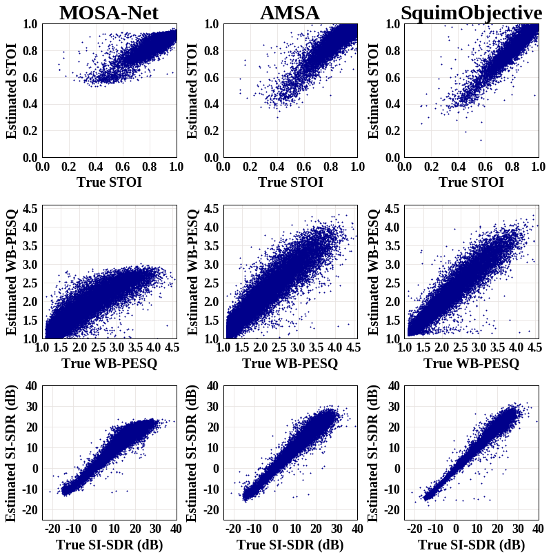
8. Comparison with ground truths and baselines

Visualizing the estimated metrics by the SquimObjective and SquimSubjective models can help users better understand how the models can be applicable in real scenario. The graph below shows scatter plots of three different systems: MOSA-Net [1], AMSA [2], and the SquimObjective model, where y axis represents the estimated STOI, PESQ, and Si-SDR scores, and x axis represents the corresponding ground truth.

[1] Zezario, Ryandhimas E., Szu-Wei Fu, Fei Chen, Chiou-Shann Fuh, Hsin-Min Wang, and Yu Tsao. “Deep learning-based non-intrusive multi-objective speech assessment model with cross-domain features.” IEEE/ACM Transactions on Audio, Speech, and Language Processing 31 (2022): 54-70.

[2] Dong, Xuan, and Donald S. Williamson. “An attention enhanced multi-task model for objective speech assessment in real-world environments.” In ICASSP 2020-2020 IEEE International Conference on Acoustics, Speech and Signal Processing (ICASSP), pp. 911-915. IEEE, 2020.

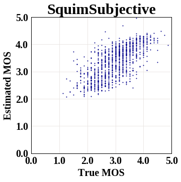
The graph below shows scatter plot of the SquimSubjective model, where y axis represents the estimated MOS metric score, and x axis represents the corresponding ground truth.