Filter design tutorial

Author: Moto Hira

This tutorial shows how to create basic digital filters (impulse responses) and their properties.

We look into low-pass, high-pass and band-pass filters based on windowed-sinc kernels, and frequency sampling method.

Warning

This tutorial requires prototype DSP features, which are available in nightly builds.

Please refer to https://pytorch.org/get-started/locally for instructions for installing a nightly build.

import torch
import torchaudio

print(torch.__version__)
print(torchaudio.__version__)

import matplotlib.pyplot as plt

2.4.0.dev20240416
2.2.0.dev20240418

from torchaudio.prototype.functional import frequency_impulse_response, sinc_impulse_response

Windowed-Sinc Filter

Sinc filter is an idealized filter which removes frequencies above the cutoff frequency without affecting the lower frequencies.

Sinc filter has infinite filter width in analytical solution. In numerical computation, sinc filter cannot be expressed exactly, so an approximation is required.

Windowed-sinc finite impulse response is an approximation of sinc filter. It is obtained by first evaluating sinc function for given cutoff frequencies, then truncating the filter skirt, and applying a window, such as Hamming window, to reduce the artifacts introduced from the truncation.

sinc_impulse_response() generates windowed-sinc impulse response for given cutoff frequencies.

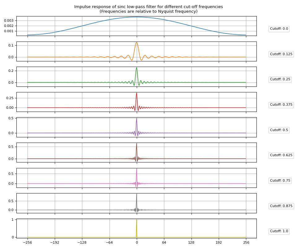
Low-pass filter

Impulse Response

Creating sinc IR is as easy as passing cutoff frequency values to sinc_impulse_response().

cutoff = torch.linspace(0.0, 1.0, 9)
irs = sinc_impulse_response(cutoff, window_size=513)

print("Cutoff shape:", cutoff.shape)
print("Impulse response shape:", irs.shape)

Cutoff shape: torch.Size([9])
Impulse response shape: torch.Size([9, 513])

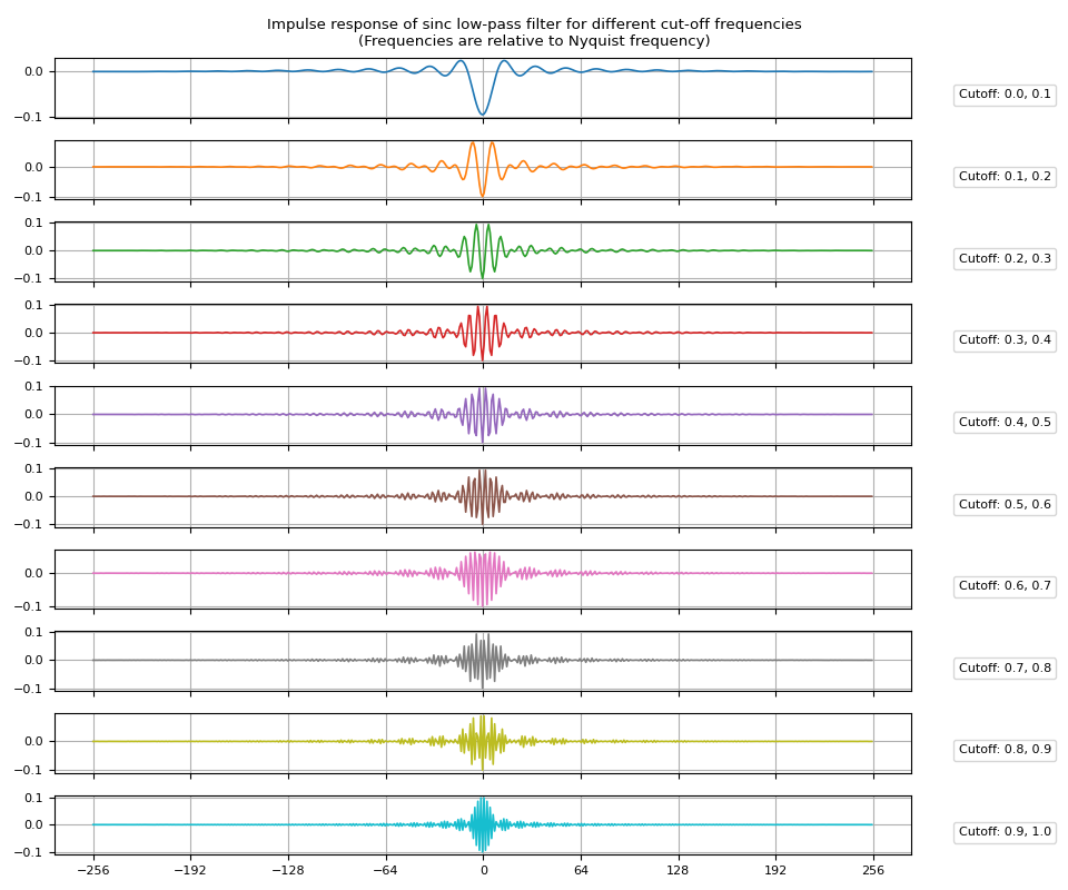
Let’s visualize the resulting impulse responses.

def plot_sinc_ir(irs, cutoff):
    num_filts, window_size = irs.shape
    half = window_size // 2

    fig, axes = plt.subplots(num_filts, 1, sharex=True, figsize=(9.6, 8))
    t = torch.linspace(-half, half - 1, window_size)
    for ax, ir, coff, color in zip(axes, irs, cutoff, plt.cm.tab10.colors):
        ax.plot(t, ir, linewidth=1.2, color=color, zorder=4, label=f"Cutoff: {coff}")
        ax.legend(loc=(1.05, 0.2), handletextpad=0, handlelength=0)
        ax.grid(True)
    fig.suptitle(
        "Impulse response of sinc low-pass filter for different cut-off frequencies\n"
        "(Frequencies are relative to Nyquist frequency)"
    )
    axes[-1].set_xticks([i * half // 4 for i in range(-4, 5)])
    fig.tight_layout()

plot_sinc_ir(irs, cutoff)

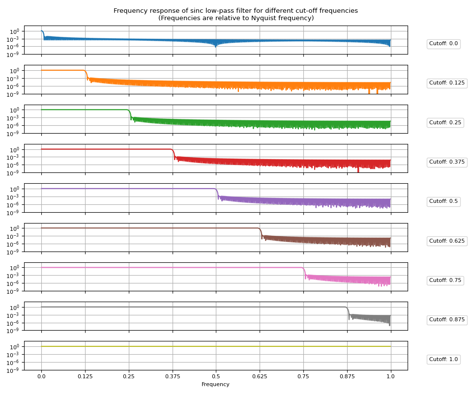
Frequency Response

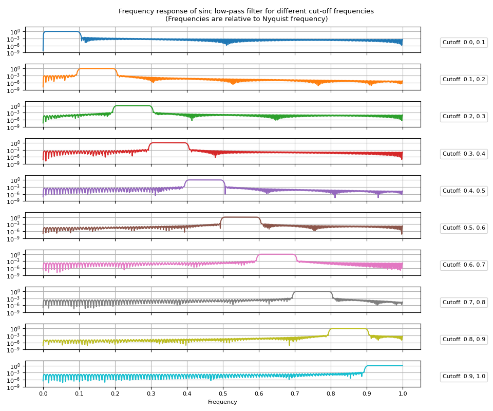
Next, let’s look at the frequency responses. Simpy applying Fourier transform to the impulse responses will give the frequency responses.

frs = torch.fft.rfft(irs, n=2048, dim=1).abs()

Let’s visualize the resulting frequency responses.

def plot_sinc_fr(frs, cutoff, band=False):
    num_filts, num_fft = frs.shape
    num_ticks = num_filts + 1 if band else num_filts

    fig, axes = plt.subplots(num_filts, 1, sharex=True, sharey=True, figsize=(9.6, 8))
    for ax, fr, coff, color in zip(axes, frs, cutoff, plt.cm.tab10.colors):
        ax.grid(True)
        ax.semilogy(fr, color=color, zorder=4, label=f"Cutoff: {coff}")
        ax.legend(loc=(1.05, 0.2), handletextpad=0, handlelength=0).set_zorder(3)
    axes[-1].set(
        ylim=[None, 100],
        yticks=[1e-9, 1e-6, 1e-3, 1],
        xticks=torch.linspace(0, num_fft, num_ticks),
        xticklabels=[f"{i/(num_ticks - 1)}" for i in range(num_ticks)],
        xlabel="Frequency",
    )
    fig.suptitle(
        "Frequency response of sinc low-pass filter for different cut-off frequencies\n"
        "(Frequencies are relative to Nyquist frequency)"
    )
    fig.tight_layout()

plot_sinc_fr(frs, cutoff)

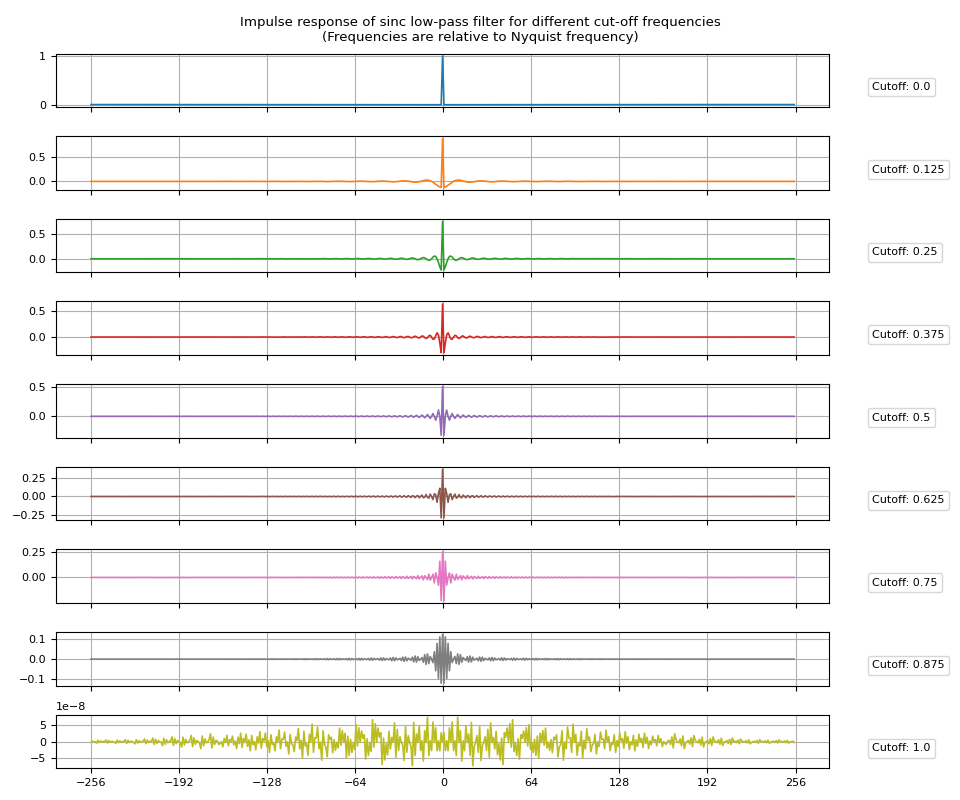
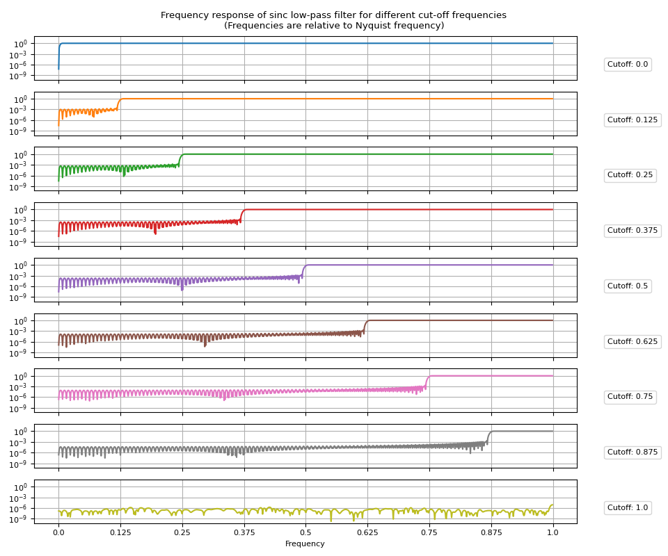
High-pass filter

High-pass filter can be obtained by subtracting low-pass impulse response from the Dirac delta function.

Passing high_pass=True to sinc_impulse_response() will change the returned filter kernel to high pass filter.

irs = sinc_impulse_response(cutoff, window_size=513, high_pass=True)
frs = torch.fft.rfft(irs, n=2048, dim=1).abs()

Impulse Response

plot_sinc_ir(irs, cutoff)

Frequency Response

plot_sinc_fr(frs, cutoff)

Band-pass filter

Band-pass filter can be obtained by subtracting low-pass filter for upper band from that of lower band.

cutoff = torch.linspace(0.0, 1, 11)
c_low = cutoff[:-1]
c_high = cutoff[1:]

irs = sinc_impulse_response(c_low, window_size=513) - sinc_impulse_response(c_high, window_size=513)
frs = torch.fft.rfft(irs, n=2048, dim=1).abs()

Impulse Response

coff = [f"{l.item():.1f}, {h.item():.1f}" for l, h in zip(c_low, c_high)]
plot_sinc_ir(irs, coff)

Frequency Response

plot_sinc_fr(frs, coff, band=True)

Frequency Sampling

The next method we look into starts from a desired frequency response and obtain impulse response by applying inverse Fourier transform.

frequency_impulse_response() takes (unnormalized) magnitude distribution of frequencies and construct impulse response from it.

Note however that the resulting impulse response does not produce the desired frequency response.

In the following, we create multiple filters and compare the input frequency response and the actual frequency response.

Brick-wall filter

Let’s start from brick-wall filter

magnitudes = torch.concat([torch.ones((128,)), torch.zeros((128,))])
ir = frequency_impulse_response(magnitudes)

print("Magnitudes:", magnitudes.shape)
print("Impulse Response:", ir.shape)

Magnitudes: torch.Size([256])
Impulse Response: torch.Size([510])

def plot_ir(magnitudes, ir, num_fft=2048):
    fr = torch.fft.rfft(ir, n=num_fft, dim=0).abs()
    ir_size = ir.size(-1)
    half = ir_size // 2

    fig, axes = plt.subplots(3, 1)
    t = torch.linspace(-half, half - 1, ir_size)
    axes[0].plot(t, ir)
    axes[0].grid(True)
    axes[0].set(title="Impulse Response")
    axes[0].set_xticks([i * half // 4 for i in range(-4, 5)])
    t = torch.linspace(0, 1, fr.numel())
    axes[1].plot(t, fr, label="Actual")
    axes[2].semilogy(t, fr, label="Actual")
    t = torch.linspace(0, 1, magnitudes.numel())
    for i in range(1, 3):
        axes[i].plot(t, magnitudes, label="Desired (input)", linewidth=1.1, linestyle="--")
        axes[i].grid(True)
    axes[1].set(title="Frequency Response")
    axes[2].set(title="Frequency Response (log-scale)", xlabel="Frequency")
    axes[2].legend(loc="center right")
    fig.tight_layout()

plot_ir(magnitudes, ir)

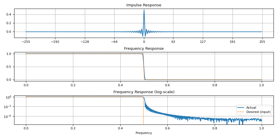
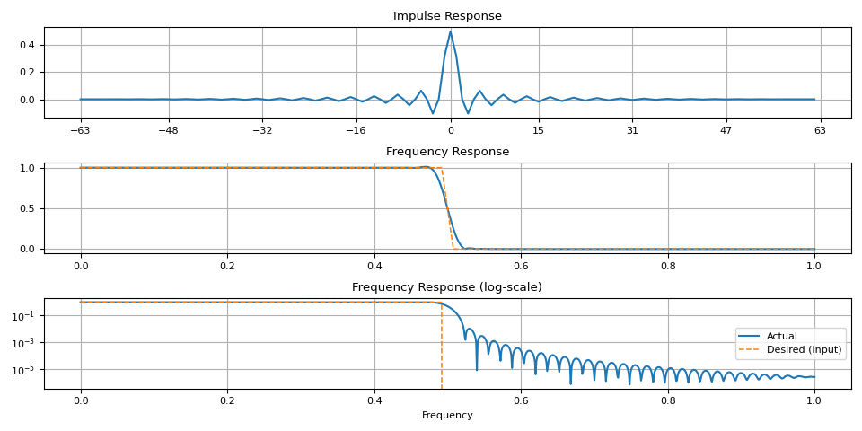
Notice that there are artifacts around the transition band. This is more noticeable when the window size is small.

magnitudes = torch.concat([torch.ones((32,)), torch.zeros((32,))])
ir = frequency_impulse_response(magnitudes)

plot_ir(magnitudes, ir)

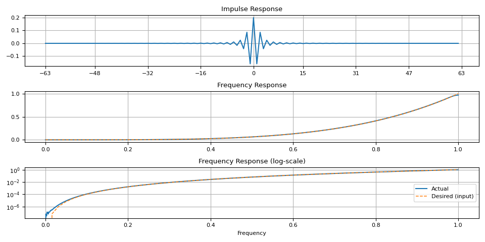
Arbitrary shapes

magnitudes = torch.linspace(0, 1, 64) ** 4.0
ir = frequency_impulse_response(magnitudes)

plot_ir(magnitudes, ir)

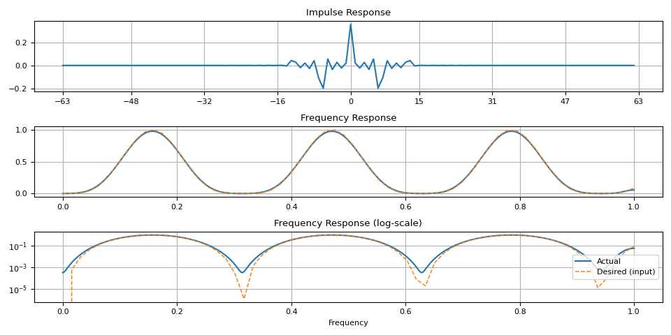
magnitudes = torch.sin(torch.linspace(0, 10, 64)) ** 4.0
ir = frequency_impulse_response(magnitudes)

plot_ir(magnitudes, ir)

References

• https://en.wikipedia.org/wiki/Sinc_filter

• https://www.analog.com/media/en/technical-documentation/dsp-book/dsp_book_Ch16.pdf

• https://courses.engr.illinois.edu/ece401/fa2020/slides/lec10.pdf

• https://ccrma.stanford.edu/~jos/sasp/Windowing_Desired_Impulse_Response.html