


Note
Click here to download the full example code
Speech Enhancement with MVDR Beamforming
Author: Zhaoheng Ni
1. Overview
This is a tutorial on applying Minimum Variance Distortionless Response (MVDR) beamforming to estimate enhanced speech with TorchAudio.
Steps:
Generate an ideal ratio mask (IRM) by dividing the clean/noise magnitude by the mixture magnitude.
Estimate power spectral density (PSD) matrices using
torchaudio.transforms.PSD().Estimate enhanced speech using MVDR modules (
torchaudio.transforms.SoudenMVDR()andtorchaudio.transforms.RTFMVDR()).Benchmark the two methods (
torchaudio.functional.rtf_evd()andtorchaudio.functional.rtf_power()) for computing the relative transfer function (RTF) matrix of the reference microphone.
import torch
import torchaudio
import torchaudio.functional as F

print(torch.__version__)
print(torchaudio.__version__)


import matplotlib.pyplot as plt
import mir_eval
from IPython.display import Audio
2.6.0.dev20241104
2.5.0.dev20241105
2. Preparation
2.1. Import the packages
First, we install and import the necessary packages.
mir_eval, pesq, and pystoi packages are required for
evaluating the speech enhancement performance.
# When running this example in notebook, install the following packages.
# !pip3 install mir_eval
# !pip3 install pesq
# !pip3 install pystoi

from pesq import pesq
from pystoi import stoi
from torchaudio.utils import download_asset
2.2. Download audio data
The multi-channel audio example is selected from ConferencingSpeech dataset.
The original filename is
SSB07200001\#noise-sound-bible-0038\#7.86_6.16_3.00_3.14_4.84_134.5285_191.7899_0.4735\#15217\#25.16333303751458\#0.2101221178590021.wav
which was generated with:
SSB07200001.wavfrom AISHELL-3 (Apache License v.2.0)noise-sound-bible-0038.wavfrom MUSAN (Attribution 4.0 International — CC BY 4.0)
SAMPLE_RATE = 16000
SAMPLE_CLEAN = download_asset("tutorial-assets/mvdr/clean_speech.wav")
SAMPLE_NOISE = download_asset("tutorial-assets/mvdr/noise.wav")
  0%|          | 0.00/0.98M [00:00<?, ?B/s]
100%|##########| 0.98M/0.98M [00:00<00:00, 86.6MB/s]

  0%|          | 0.00/1.95M [00:00<?, ?B/s]
100%|##########| 1.95M/1.95M [00:00<00:00, 67.7MB/s]
2.3. Helper functions
def plot_spectrogram(stft, title="Spectrogram"):
    magnitude = stft.abs()
    spectrogram = 20 * torch.log10(magnitude + 1e-8).numpy()
    figure, axis = plt.subplots(1, 1)
    img = axis.imshow(spectrogram, cmap="viridis", vmin=-100, vmax=0, origin="lower", aspect="auto")
    axis.set_title(title)
    plt.colorbar(img, ax=axis)


def plot_mask(mask, title="Mask"):
    mask = mask.numpy()
    figure, axis = plt.subplots(1, 1)
    img = axis.imshow(mask, cmap="viridis", origin="lower", aspect="auto")
    axis.set_title(title)
    plt.colorbar(img, ax=axis)


def si_snr(estimate, reference, epsilon=1e-8):
    estimate = estimate - estimate.mean()
    reference = reference - reference.mean()
    reference_pow = reference.pow(2).mean(axis=1, keepdim=True)
    mix_pow = (estimate * reference).mean(axis=1, keepdim=True)
    scale = mix_pow / (reference_pow + epsilon)

    reference = scale * reference
    error = estimate - reference

    reference_pow = reference.pow(2)
    error_pow = error.pow(2)

    reference_pow = reference_pow.mean(axis=1)
    error_pow = error_pow.mean(axis=1)

    si_snr = 10 * torch.log10(reference_pow) - 10 * torch.log10(error_pow)
    return si_snr.item()


def generate_mixture(waveform_clean, waveform_noise, target_snr):
    power_clean_signal = waveform_clean.pow(2).mean()
    power_noise_signal = waveform_noise.pow(2).mean()
    current_snr = 10 * torch.log10(power_clean_signal / power_noise_signal)
    waveform_noise *= 10 ** (-(target_snr - current_snr) / 20)
    return waveform_clean + waveform_noise


def evaluate(estimate, reference):
    si_snr_score = si_snr(estimate, reference)
    (
        sdr,
        _,
        _,
        _,
    ) = mir_eval.separation.bss_eval_sources(reference.numpy(), estimate.numpy(), False)
    pesq_mix = pesq(SAMPLE_RATE, estimate[0].numpy(), reference[0].numpy(), "wb")
    stoi_mix = stoi(reference[0].numpy(), estimate[0].numpy(), SAMPLE_RATE, extended=False)
    print(f"SDR score: {sdr[0]}")
    print(f"Si-SNR score: {si_snr_score}")
    print(f"PESQ score: {pesq_mix}")
    print(f"STOI score: {stoi_mix}")
3. Generate Ideal Ratio Masks (IRMs)
3.1. Load audio data
waveform_clean, sr = torchaudio.load(SAMPLE_CLEAN)
waveform_noise, sr2 = torchaudio.load(SAMPLE_NOISE)
assert sr == sr2 == SAMPLE_RATE
# The mixture waveform is a combination of clean and noise waveforms with a desired SNR.
target_snr = 3
waveform_mix = generate_mixture(waveform_clean, waveform_noise, target_snr)
Note: To improve computational robustness, it is recommended to represent
the waveforms as double-precision floating point (torch.float64 or torch.double) values.
3.2. Compute STFT coefficients
N_FFT = 1024
N_HOP = 256
stft = torchaudio.transforms.Spectrogram(
    n_fft=N_FFT,
    hop_length=N_HOP,
    power=None,
)
istft = torchaudio.transforms.InverseSpectrogram(n_fft=N_FFT, hop_length=N_HOP)

stft_mix = stft(waveform_mix)
stft_clean = stft(waveform_clean)
stft_noise = stft(waveform_noise)
3.2.1. Visualize mixture speech
We evaluate the quality of the mixture speech or the enhanced speech using the following three metrics:
signal-to-distortion ratio (SDR)
scale-invariant signal-to-noise ratio (Si-SNR, or Si-SDR in some papers)
Perceptual Evaluation of Speech Quality (PESQ)
We also evaluate the intelligibility of the speech with the Short-Time Objective Intelligibility (STOI) metric.
plot_spectrogram(stft_mix[0], "Spectrogram of Mixture Speech (dB)")
evaluate(waveform_mix[0:1], waveform_clean[0:1])
Audio(waveform_mix[0], rate=SAMPLE_RATE)
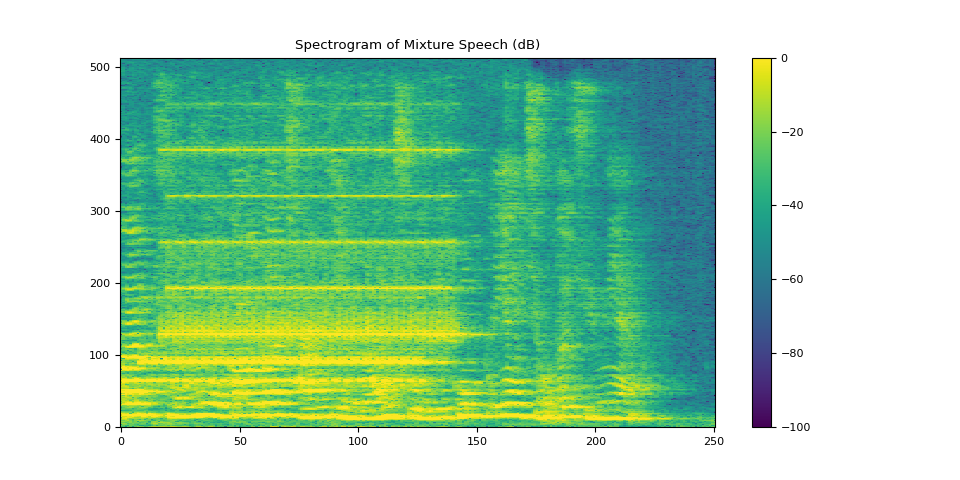
SDR score: 4.140362181778018
Si-SNR score: 4.104058905536078
PESQ score: 2.0084526538848877
STOI score: 0.7724339398714715
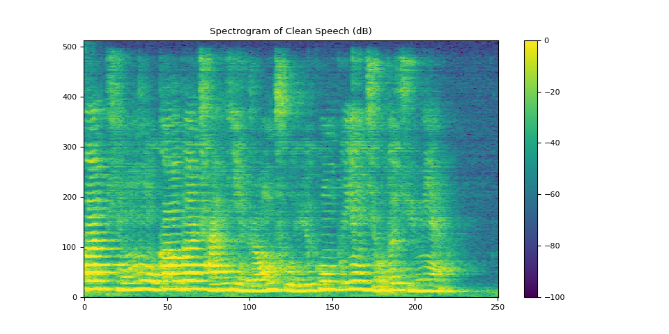
3.2.2. Visualize clean speech
plot_spectrogram(stft_clean[0], "Spectrogram of Clean Speech (dB)")
Audio(waveform_clean[0], rate=SAMPLE_RATE)
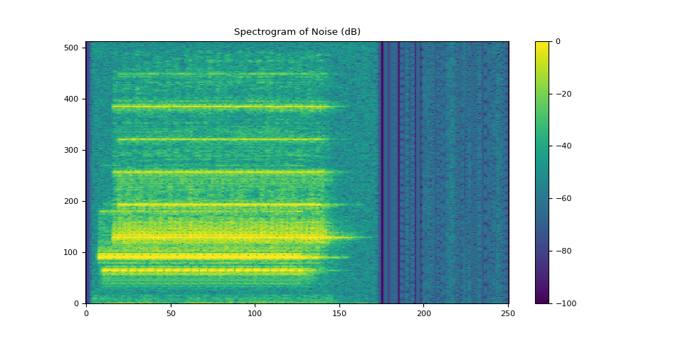
3.2.3. Visualize noise
plot_spectrogram(stft_noise[0], "Spectrogram of Noise (dB)")
Audio(waveform_noise[0], rate=SAMPLE_RATE)
3.3. Define the reference microphone
We choose the first microphone in the array as the reference channel for demonstration. The selection of the reference channel may depend on the design of the microphone array.
You can also apply an end-to-end neural network which estimates both the reference channel and the PSD matrices, then obtains the enhanced STFT coefficients by the MVDR module.
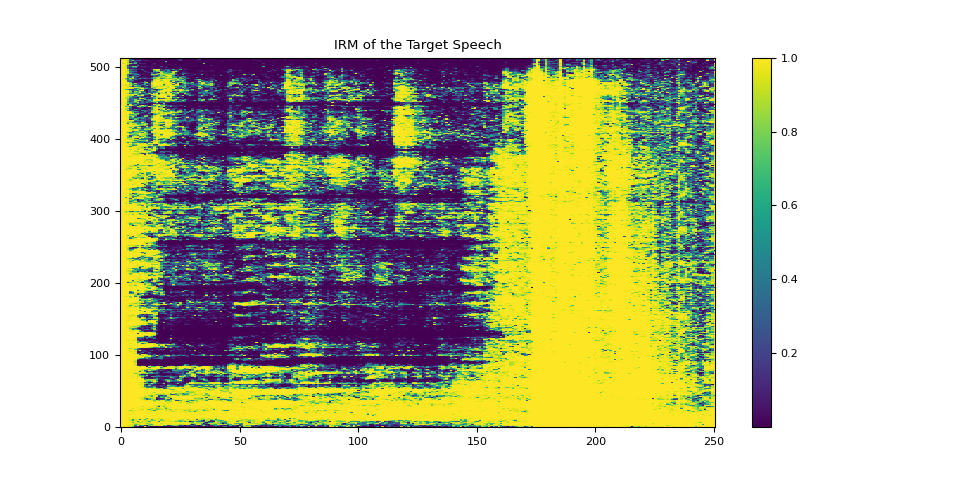
3.4. Compute IRMs
def get_irms(stft_clean, stft_noise):
    mag_clean = stft_clean.abs() ** 2
    mag_noise = stft_noise.abs() ** 2
    irm_speech = mag_clean / (mag_clean + mag_noise)
    irm_noise = mag_noise / (mag_clean + mag_noise)
    return irm_speech[REFERENCE_CHANNEL], irm_noise[REFERENCE_CHANNEL]


irm_speech, irm_noise = get_irms(stft_clean, stft_noise)
3.4.1. Visualize IRM of target speech
plot_mask(irm_speech, "IRM of the Target Speech")
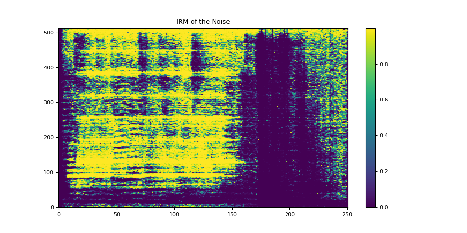
3.4.2. Visualize IRM of noise
plot_mask(irm_noise, "IRM of the Noise")
4. Compute PSD matrices
torchaudio.transforms.PSD() computes the time-invariant PSD matrix given
the multi-channel complex-valued STFT coefficients of the mixture speech
and the time-frequency mask.
The shape of the PSD matrix is (…, freq, channel, channel).
psd_transform = torchaudio.transforms.PSD()

psd_speech = psd_transform(stft_mix, irm_speech)
psd_noise = psd_transform(stft_mix, irm_noise)
5. Beamforming using SoudenMVDR
5.1. Apply beamforming
torchaudio.transforms.SoudenMVDR() takes the multi-channel
complexed-valued STFT coefficients of the mixture speech, PSD matrices of
target speech and noise, and the reference channel inputs.
The output is a single-channel complex-valued STFT coefficients of the enhanced speech.
We can then obtain the enhanced waveform by passing this output to the
torchaudio.transforms.InverseSpectrogram() module.
mvdr_transform = torchaudio.transforms.SoudenMVDR()
stft_souden = mvdr_transform(stft_mix, psd_speech, psd_noise, reference_channel=REFERENCE_CHANNEL)
waveform_souden = istft(stft_souden, length=waveform_mix.shape[-1])
5.2. Result for SoudenMVDR
plot_spectrogram(stft_souden, "Enhanced Spectrogram by SoudenMVDR (dB)")
waveform_souden = waveform_souden.reshape(1, -1)
evaluate(waveform_souden, waveform_clean[0:1])
Audio(waveform_souden, rate=SAMPLE_RATE)
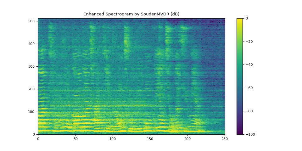
SDR score: 17.946234447508765
Si-SNR score: 12.215202612266587
PESQ score: 3.3447437286376953
STOI score: 0.8712864479161743
6. Beamforming using RTFMVDR
6.1. Compute RTF
TorchAudio offers two methods for computing the RTF matrix of a target speech:
torchaudio.functional.rtf_evd(), which applies eigenvalue decomposition to the PSD matrix of target speech to get the RTF matrix.torchaudio.functional.rtf_power(), which applies the power iteration method. You can specify the number of iterations with argumentn_iter.
rtf_evd = F.rtf_evd(psd_speech)
rtf_power = F.rtf_power(psd_speech, psd_noise, reference_channel=REFERENCE_CHANNEL)
6.2. Apply beamforming
torchaudio.transforms.RTFMVDR() takes the multi-channel
complexed-valued STFT coefficients of the mixture speech, RTF matrix of target speech,
PSD matrix of noise, and the reference channel inputs.
The output is a single-channel complex-valued STFT coefficients of the enhanced speech.
We can then obtain the enhanced waveform by passing this output to the
torchaudio.transforms.InverseSpectrogram() module.
mvdr_transform = torchaudio.transforms.RTFMVDR()

# compute the enhanced speech based on F.rtf_evd
stft_rtf_evd = mvdr_transform(stft_mix, rtf_evd, psd_noise, reference_channel=REFERENCE_CHANNEL)
waveform_rtf_evd = istft(stft_rtf_evd, length=waveform_mix.shape[-1])

# compute the enhanced speech based on F.rtf_power
stft_rtf_power = mvdr_transform(stft_mix, rtf_power, psd_noise, reference_channel=REFERENCE_CHANNEL)
waveform_rtf_power = istft(stft_rtf_power, length=waveform_mix.shape[-1])
6.3. Result for RTFMVDR with rtf_evd
plot_spectrogram(stft_rtf_evd, "Enhanced Spectrogram by RTFMVDR and F.rtf_evd (dB)")
waveform_rtf_evd = waveform_rtf_evd.reshape(1, -1)
evaluate(waveform_rtf_evd, waveform_clean[0:1])
Audio(waveform_rtf_evd, rate=SAMPLE_RATE)
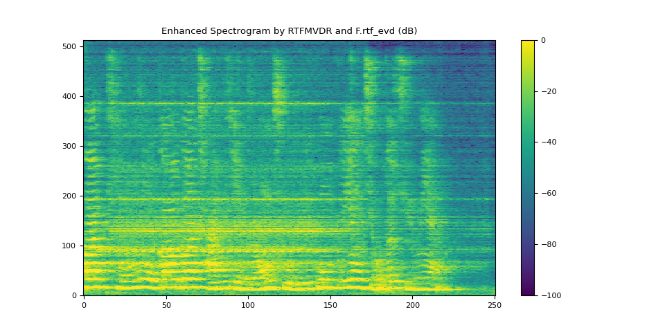
SDR score: 11.880210635280273
Si-SNR score: 10.714419996128061
PESQ score: 3.083890914916992
STOI score: 0.8261544910053075
6.4. Result for RTFMVDR with rtf_power
plot_spectrogram(stft_rtf_power, "Enhanced Spectrogram by RTFMVDR and F.rtf_power (dB)")
waveform_rtf_power = waveform_rtf_power.reshape(1, -1)
evaluate(waveform_rtf_power, waveform_clean[0:1])
Audio(waveform_rtf_power, rate=SAMPLE_RATE)
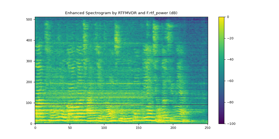
SDR score: 15.424590276934103
Si-SNR score: 13.035440892133451
PESQ score: 3.487997531890869
STOI score: 0.8798278461896808
Total running time of the script: ( 0 minutes 1.956 seconds)
