Audio Resampling

Author: Caroline Chen, Moto Hira

This tutorial shows how to use torchaudio’s resampling API.

import torch
import torchaudio
import torchaudio.functional as F
import torchaudio.transforms as T

print(torch.__version__)
print(torchaudio.__version__)

2.0.0
2.0.1

Preparation

First, we import the modules and define the helper functions.

import math
import timeit

import librosa
import resampy
import matplotlib.pyplot as plt
import matplotlib.colors as mcolors
import pandas as pd
from IPython.display import Audio, display

pd.set_option('display.max_rows', None)
pd.set_option('display.max_columns', None)

DEFAULT_OFFSET = 201


def _get_log_freq(sample_rate, max_sweep_rate, offset):
    """Get freqs evenly spaced out in log-scale, between [0, max_sweep_rate // 2]

    offset is used to avoid negative infinity `log(offset + x)`.

    """
    start, stop = math.log(offset), math.log(offset + max_sweep_rate // 2)
    return torch.exp(torch.linspace(start, stop, sample_rate, dtype=torch.double)) - offset


def _get_inverse_log_freq(freq, sample_rate, offset):
    """Find the time where the given frequency is given by _get_log_freq"""
    half = sample_rate // 2
    return sample_rate * (math.log(1 + freq / offset) / math.log(1 + half / offset))


def _get_freq_ticks(sample_rate, offset, f_max):
    # Given the original sample rate used for generating the sweep,
    # find the x-axis value where the log-scale major frequency values fall in
    times, freq = [], []
    for exp in range(2, 5):
        for v in range(1, 10):
            f = v * 10**exp
            if f < sample_rate // 2:
                t = _get_inverse_log_freq(f, sample_rate, offset) / sample_rate
                times.append(t)
                freq.append(f)
    t_max = _get_inverse_log_freq(f_max, sample_rate, offset) / sample_rate
    times.append(t_max)
    freq.append(f_max)
    return times, freq


def get_sine_sweep(sample_rate, offset=DEFAULT_OFFSET):
    max_sweep_rate = sample_rate
    freq = _get_log_freq(sample_rate, max_sweep_rate, offset)
    delta = 2 * math.pi * freq / sample_rate
    cummulative = torch.cumsum(delta, dim=0)
    signal = torch.sin(cummulative).unsqueeze(dim=0)
    return signal


def plot_sweep(
    waveform,
    sample_rate,
    title,
    max_sweep_rate=48000,
    offset=DEFAULT_OFFSET,
):
    x_ticks = [100, 500, 1000, 5000, 10000, 20000, max_sweep_rate // 2]
    y_ticks = [1000, 5000, 10000, 20000, sample_rate // 2]

    time, freq = _get_freq_ticks(max_sweep_rate, offset, sample_rate // 2)
    freq_x = [f if f in x_ticks and f <= max_sweep_rate // 2 else None for f in freq]
    freq_y = [f for f in freq if f in y_ticks and 1000 <= f <= sample_rate // 2]

    figure, axis = plt.subplots(1, 1)
    _, _, _, cax = axis.specgram(waveform[0].numpy(), Fs=sample_rate)
    plt.xticks(time, freq_x)
    plt.yticks(freq_y, freq_y)
    axis.set_xlabel("Original Signal Frequency (Hz, log scale)")
    axis.set_ylabel("Waveform Frequency (Hz)")
    axis.xaxis.grid(True, alpha=0.67)
    axis.yaxis.grid(True, alpha=0.67)
    figure.suptitle(f"{title} (sample rate: {sample_rate} Hz)")
    plt.colorbar(cax)
    plt.show(block=True)

Resampling Overview

To resample an audio waveform from one freqeuncy to another, you can use torchaudio.transforms.Resample or torchaudio.functional.resample(). transforms.Resample precomputes and caches the kernel used for resampling, while functional.resample computes it on the fly, so using torchaudio.transforms.Resample will result in a speedup when resampling multiple waveforms using the same parameters (see Benchmarking section).

Both resampling methods use bandlimited sinc interpolation to compute signal values at arbitrary time steps. The implementation involves convolution, so we can take advantage of GPU / multithreading for performance improvements.

Note

When using resampling in multiple subprocesses, such as data loading with multiple worker processes, your application might create more threads than your system can handle efficiently. Setting torch.set_num_threads(1) might help in this case.

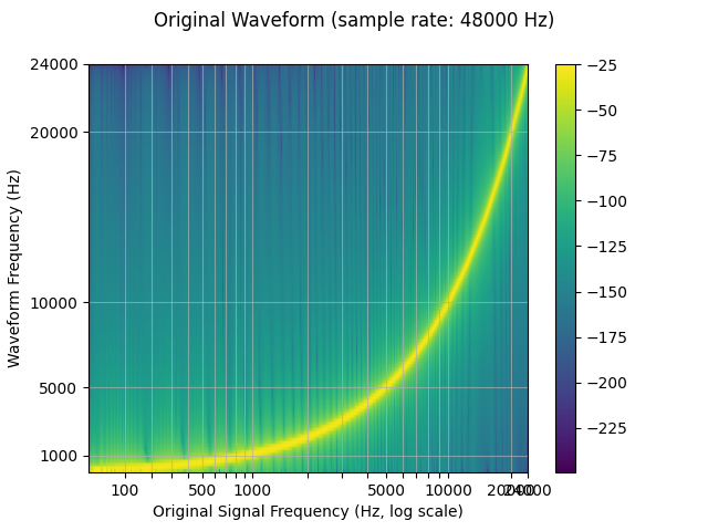
Because a finite number of samples can only represent a finite number of frequencies, resampling does not produce perfect results, and a variety of parameters can be used to control for its quality and computational speed. We demonstrate these properties through resampling a logarithmic sine sweep, which is a sine wave that increases exponentially in frequency over time.

The spectrograms below show the frequency representation of the signal, where the x-axis corresponds to the frequency of the original waveform (in log scale), y-axis the frequency of the plotted waveform, and color intensity the amplitude.

sample_rate = 48000
waveform = get_sine_sweep(sample_rate)

plot_sweep(waveform, sample_rate, title="Original Waveform")
Audio(waveform.numpy()[0], rate=sample_rate)

Now we resample (downsample) it.

We see that in the spectrogram of the resampled waveform, there is an artifact, which was not present in the original waveform. This effect is called aliasing. This page has an explanation of how it happens, and why it looks like a reflection.

resample_rate = 32000
resampler = T.Resample(sample_rate, resample_rate, dtype=waveform.dtype)
resampled_waveform = resampler(waveform)

plot_sweep(resampled_waveform, resample_rate, title="Resampled Waveform")
Audio(resampled_waveform.numpy()[0], rate=resample_rate)

Controling resampling quality with parameters

Lowpass filter width

Because the filter used for interpolation extends infinitely, the lowpass_filter_width parameter is used to control for the width of the filter to use to window the interpolation. It is also referred to as the number of zero crossings, since the interpolation passes through zero at every time unit. Using a larger lowpass_filter_width provides a sharper, more precise filter, but is more computationally expensive.

sample_rate = 48000
resample_rate = 32000

resampled_waveform = F.resample(waveform, sample_rate, resample_rate, lowpass_filter_width=6)
plot_sweep(resampled_waveform, resample_rate, title="lowpass_filter_width=6")

resampled_waveform = F.resample(waveform, sample_rate, resample_rate, lowpass_filter_width=128)
plot_sweep(resampled_waveform, resample_rate, title="lowpass_filter_width=128")

Rolloff

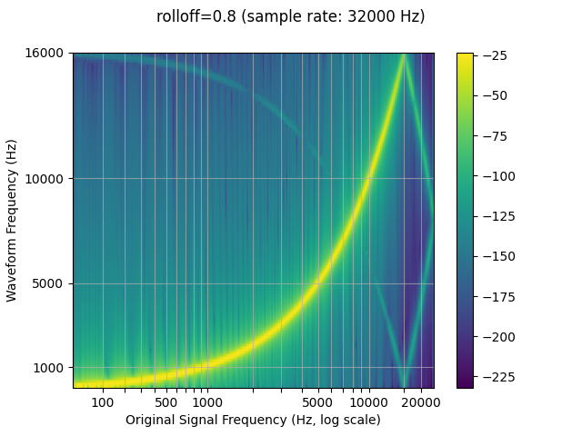
The rolloff parameter is represented as a fraction of the Nyquist frequency, which is the maximal frequency representable by a given finite sample rate. rolloff determines the lowpass filter cutoff and controls the degree of aliasing, which takes place when frequencies higher than the Nyquist are mapped to lower frequencies. A lower rolloff will therefore reduce the amount of aliasing, but it will also reduce some of the higher frequencies.

sample_rate = 48000
resample_rate = 32000

resampled_waveform = F.resample(waveform, sample_rate, resample_rate, rolloff=0.99)
plot_sweep(resampled_waveform, resample_rate, title="rolloff=0.99")

resampled_waveform = F.resample(waveform, sample_rate, resample_rate, rolloff=0.8)
plot_sweep(resampled_waveform, resample_rate, title="rolloff=0.8")

Window function

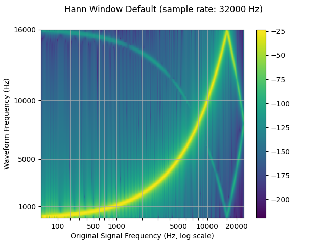
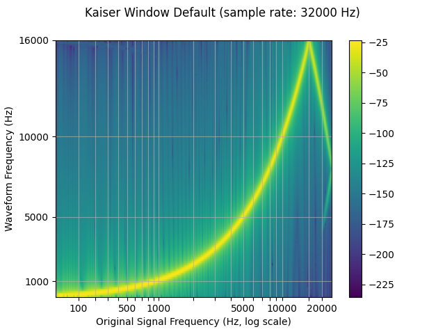
By default, torchaudio’s resample uses the Hann window filter, which is a weighted cosine function. It additionally supports the Kaiser window, which is a near optimal window function that contains an additional beta parameter that allows for the design of the smoothness of the filter and width of impulse. This can be controlled using the resampling_method parameter.

sample_rate = 48000
resample_rate = 32000

resampled_waveform = F.resample(waveform, sample_rate, resample_rate, resampling_method="sinc_interp_hann")
plot_sweep(resampled_waveform, resample_rate, title="Hann Window Default")

resampled_waveform = F.resample(waveform, sample_rate, resample_rate, resampling_method="sinc_interp_kaiser")
plot_sweep(resampled_waveform, resample_rate, title="Kaiser Window Default")

Comparison against librosa

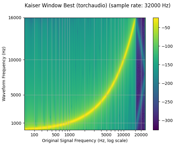
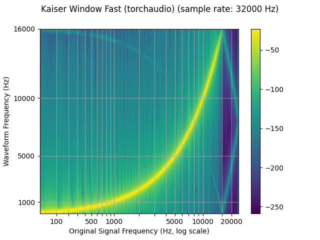
torchaudio’s resample function can be used to produce results similar to that of librosa (resampy)’s kaiser window resampling, with some noise

sample_rate = 48000
resample_rate = 32000

kaiser_best

resampled_waveform = F.resample(
    waveform,
    sample_rate,
    resample_rate,
    lowpass_filter_width=64,
    rolloff=0.9475937167399596,
    resampling_method="sinc_interp_kaiser",
    beta=14.769656459379492,
)
plot_sweep(resampled_waveform, resample_rate, title="Kaiser Window Best (torchaudio)")

librosa_resampled_waveform = torch.from_numpy(
    librosa.resample(waveform.squeeze().numpy(), orig_sr=sample_rate, target_sr=resample_rate, res_type="kaiser_best")
).unsqueeze(0)
plot_sweep(librosa_resampled_waveform, resample_rate, title="Kaiser Window Best (librosa)")

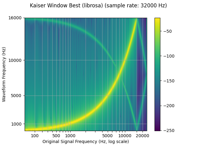
mse = torch.square(resampled_waveform - librosa_resampled_waveform).mean().item()
print("torchaudio and librosa kaiser best MSE:", mse)

torchaudio and librosa kaiser best MSE: 2.080690115366008e-06

kaiser_fast

resampled_waveform = F.resample(
    waveform,
    sample_rate,
    resample_rate,
    lowpass_filter_width=16,
    rolloff=0.85,
    resampling_method="sinc_interp_kaiser",
    beta=8.555504641634386,
)
plot_sweep(resampled_waveform, resample_rate, title="Kaiser Window Fast (torchaudio)")

librosa_resampled_waveform = torch.from_numpy(
    librosa.resample(waveform.squeeze().numpy(), orig_sr=sample_rate, target_sr=resample_rate, res_type="kaiser_fast")
).unsqueeze(0)
plot_sweep(librosa_resampled_waveform, resample_rate, title="Kaiser Window Fast (librosa)")

mse = torch.square(resampled_waveform - librosa_resampled_waveform).mean().item()
print("torchaudio and librosa kaiser fast MSE:", mse)

torchaudio and librosa kaiser fast MSE: 2.5200744248601437e-05

Performance Benchmarking

Below are benchmarks for downsampling and upsampling waveforms between two pairs of sampling rates. We demonstrate the performance implications that the lowpass_filter_wdith, window type, and sample rates can have. Additionally, we provide a comparison against librosa’s kaiser_best and kaiser_fast using their corresponding parameters in torchaudio.

print(f"torchaudio: {torchaudio.__version__}")
print(f"librosa: {librosa.__version__}")
print(f"resampy: {resampy.__version__}")

torchaudio: 2.0.1
librosa: 0.10.0
resampy: 0.2.2

def benchmark_resample_functional(
    waveform,
    sample_rate,
    resample_rate,
    lowpass_filter_width=6,
    rolloff=0.99,
    resampling_method="sinc_interp_hann",
    beta=None,
    iters=5,
):
    return timeit.timeit(
        stmt='''
torchaudio.functional.resample(
    waveform,
    sample_rate,
    resample_rate,
    lowpass_filter_width=lowpass_filter_width,
    rolloff=rolloff,
    resampling_method=resampling_method,
    beta=beta,
)
        ''',
        setup='import torchaudio',
        number=iters,
        globals=locals(),
    ) * 1000 / iters

def benchmark_resample_transforms(
    waveform,
    sample_rate,
    resample_rate,
    lowpass_filter_width=6,
    rolloff=0.99,
    resampling_method="sinc_interp_hann",
    beta=None,
    iters=5,
):
    return timeit.timeit(
        stmt='resampler(waveform)',
        setup='''
import torchaudio

resampler = torchaudio.transforms.Resample(
    sample_rate,
    resample_rate,
    lowpass_filter_width=lowpass_filter_width,
    rolloff=rolloff,
    resampling_method=resampling_method,
    dtype=waveform.dtype,
    beta=beta,
)
resampler.to(waveform.device)
        ''',
        number=iters,
        globals=locals(),
    ) * 1000 / iters

def benchmark_resample_librosa(
    waveform,
    sample_rate,
    resample_rate,
    res_type=None,
    iters=5,
):
    waveform_np = waveform.squeeze().numpy()
    return timeit.timeit(
        stmt='''
librosa.resample(
    waveform_np,
    orig_sr=sample_rate,
    target_sr=resample_rate,
    res_type=res_type,
)
        ''',
        setup='import librosa',
        number=iters,
        globals=locals(),
    ) * 1000 / iters

def benchmark(sample_rate, resample_rate):
    times, rows = [], []
    waveform = get_sine_sweep(sample_rate).to(torch.float32)

    args = (waveform, sample_rate, resample_rate)

    # sinc 64 zero-crossings
    f_time = benchmark_resample_functional(*args, lowpass_filter_width=64)
    t_time = benchmark_resample_transforms(*args, lowpass_filter_width=64)
    times.append([None, f_time, t_time])
    rows.append("sinc (width 64)")

    # sinc 6 zero-crossings
    f_time = benchmark_resample_functional(*args, lowpass_filter_width=16)
    t_time = benchmark_resample_transforms(*args, lowpass_filter_width=16)
    times.append([None, f_time, t_time])
    rows.append("sinc (width 16)")

    # kaiser best
    kwargs = {
        "lowpass_filter_width": 64,
        "rolloff": 0.9475937167399596,
        "resampling_method": "sinc_interp_kaiser",
        "beta": 14.769656459379492,
    }
    lib_time = benchmark_resample_librosa(*args, res_type="kaiser_best")
    f_time = benchmark_resample_functional(*args, **kwargs)
    t_time = benchmark_resample_transforms(*args, **kwargs)
    times.append([lib_time, f_time, t_time])
    rows.append("kaiser_best")

    # kaiser fast
    kwargs = {
        "lowpass_filter_width": 16,
        "rolloff": 0.85,
        "resampling_method": "sinc_interp_kaiser",
        "beta": 8.555504641634386,
    }
    lib_time = benchmark_resample_librosa(*args, res_type="kaiser_fast")
    f_time = benchmark_resample_functional(*args, **kwargs)
    t_time = benchmark_resample_transforms(*args, **kwargs)
    times.append([lib_time, f_time, t_time])
    rows.append("kaiser_fast")

    df = pd.DataFrame(times, columns=["librosa", "functional", "transforms"], index=rows)
    return df

def plot(df):
    print(df.round(2))
    ax = df.plot(kind="bar")
    plt.ylabel("Time Elapsed [ms]")
    plt.xticks(rotation = 0, fontsize=10)
    for cont, col, color in zip(ax.containers, df.columns, mcolors.TABLEAU_COLORS):
        label = ["N/A" if v != v else str(v) for v in df[col].round(2)]
        ax.bar_label(cont, labels=label, color=color, fontweight="bold", fontsize="x-small")

Downsample (48 -> 44.1 kHz)

df = benchmark(48_000, 44_100)
plot(df)

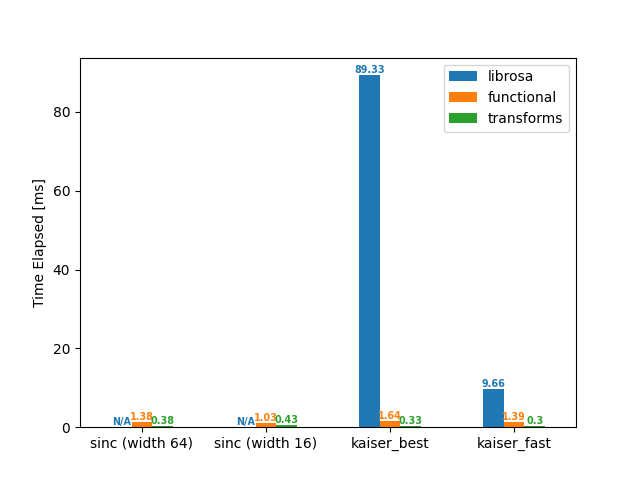
                 librosa  functional  transforms
sinc (width 64)      NaN        1.38        0.38
sinc (width 16)      NaN        1.03        0.43
kaiser_best        89.33        1.64        0.33
kaiser_fast         9.66        1.39        0.30

Downsample (16 -> 8 kHz)

df = benchmark(16_000, 8_000)
plot(df)

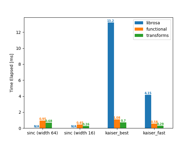
                 librosa  functional  transforms
sinc (width 64)      NaN        0.95        0.68
sinc (width 16)      NaN        0.45        0.26
kaiser_best        13.20        1.08        0.70
kaiser_fast         4.15        0.58        0.29

Upsample (44.1 -> 48 kHz)

df = benchmark(44_100, 48_000)
plot(df)

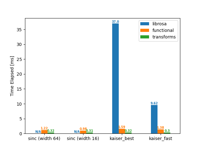
                 librosa  functional  transforms
sinc (width 64)      NaN        1.22        0.32
sinc (width 16)      NaN        0.98        0.31
kaiser_best        37.00        1.59        0.32
kaiser_fast         9.62        1.38        0.30

Upsample (8 -> 16 kHz)

df = benchmark(8_000, 16_000)
plot(df)

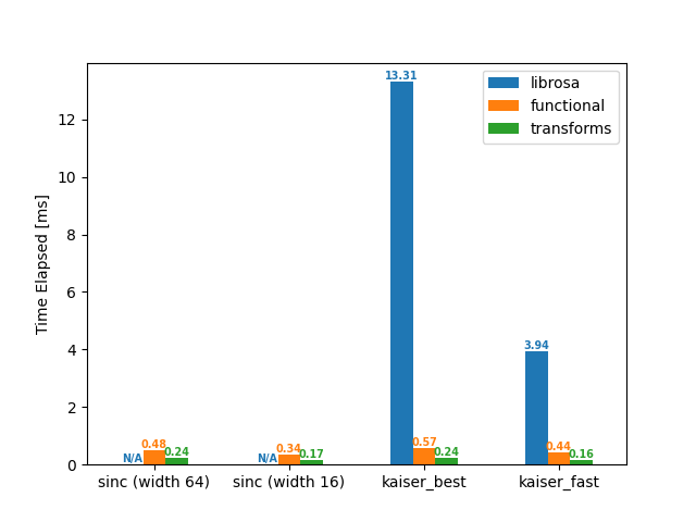
                 librosa  functional  transforms
sinc (width 64)      NaN        0.48        0.24
sinc (width 16)      NaN        0.34        0.17
kaiser_best        13.31        0.57        0.24
kaiser_fast         3.94        0.44        0.16

Summary

To elaborate on the results:

• a larger lowpass_filter_width results in a larger resampling kernel, and therefore increases computation time for both the kernel computation and convolution

• using sinc_interp_kaiser results in longer computation times than the default sinc_interp_hann because it is more complex to compute the intermediate window values

• a large GCD between the sample and resample rate will result in a simplification that allows for a smaller kernel and faster kernel computation.