TorchRec Concepts

In this section, we will learn about the key concepts of TorchRec, designed to optimize large-scale recommendation systems using PyTorch. We will learn how each concept works in detail and review how it is used with the rest of TorchRec.

TorchRec has specific input/output data types of its modules to efficiently represent sparse features, including:

• JaggedTensor: a wrapper around the lengths/offsets and values tensors for a singular sparse feature.

• KeyedJaggedTensor: efficiently represent multiple sparse features, can think of it as multiple JaggedTensors.

• KeyedTensor: a wrapper around torch.Tensor that allows access to tensor values through keys.

With the goal of high performance and efficiency, the canonical torch.Tensor is highly inefficient for representing sparse data. TorchRec introduces these new data types because they provide efficient storage and representation of sparse input data. As you will see later on, the KeyedJaggedTensor makes communication of input data in a distributed environment very efficient leading to one of the key performance advantages that TorchRec provides.

In the end-to-end training loop, TorchRec comprises of the following main components:

• Planner: Takes in the configuration of embedding tables, environment setup, and generates an optimized sharding plan for the model.

• Sharder: Shards model according to sharding plan with different sharding strategies including data-parallel, table-wise, row-wise, table-wise-row-wise, column-wise, and table-wise-column-wise sharding.

• DistributedModelParallel: Combines sharder, optimizer, and provides an entry point into the training the model in a distributed manner.

JaggedTensor

A JaggedTensor represents a sparse feature through lengths, values, and offsets. It is called “jagged” because it efficiently represents data with variable-length sequences. In contrast, a canonical torch.Tensor assumes that each sequence has the same length, which is often not the case with real world data. A JaggedTensor facilitates the representation of such data without padding making it highly efficient.

Key Components:

• Lengths: A list of integers representing the number of elements for each entity.

• Offsets: A list of integers representing the starting index of each sequence in the flattened values tensor. These provide an alternative to lengths.

• Values: A 1D tensor containing the actual values for each entity, stored contiguously.

Here is a simple example demonstrating how each of the components would look like:

# User interactions:
# - User 1 interacted with 2 items
# - User 2 interacted with 3 items
# - User 3 interacted with 1 item
lengths = [2, 3, 1]
offsets = [0, 2, 5]  # Starting index of each user's interactions
values = torch.Tensor([101, 102, 201, 202, 203, 301])  # Item IDs interacted with
jt = JaggedTensor(lengths=lengths, values=values)
# OR
jt = JaggedTensor(offsets=offsets, values=values)

KeyedJaggedTensor

A KeyedJaggedTensor extends the functionality of JaggedTensor by introducing keys (which are typically feature names) to label different groups of features, for example, user features and item features. This is the data type used in forward of EmbeddingBagCollection and EmbeddingCollection as they are used to represent multiple features in a table.

A KeyedJaggedTensor has an implied batch size, which is the number of features divided by the length of lengths tensor. The example below has a batch size of 2. Similar to a JaggedTensor, the offsets and lengths function in the same manner. You can also access the lengths, offsets, and values of a feature by accessing the key from the KeyedJaggedTensor.

keys = ["user_features", "item_features"]
# Lengths of interactions:
# - User features: 2 users, with 2 and 3 interactions respectively
# - Item features: 2 items, with 1 and 2 interactions respectively
lengths = [2, 3, 1, 2]
values = torch.Tensor([11, 12, 21, 22, 23, 101, 102, 201])
# Create a KeyedJaggedTensor
kjt = KeyedJaggedTensor(keys=keys, lengths=lengths, values=values)
# Access the features by key
print(kjt["user_features"])
# Outputs user features
print(kjt["item_features"])

Planner

The TorchRec planner helps determine the best sharding configuration for a model. It evaluates multiple possibilities for sharding embedding tables and optimizes for performance. The planner performs the following:

• Assesses the memory constraints of the hardware.

• Estimates compute requirements based on memory fetches, such as embedding lookups.

• Addresses data-specific factors.

• Considers other hardware specifics, such as bandwidth, to generate an optimal sharding plan.

To ensure accurate consideration of these factors, the Planner can incorporate data about the embedding tables, constraints, hardware information, and topology to help in generating an optimal plan.

Sharding of EmbeddingTables

TorchRec sharder provides multiple sharding strategies for various use cases, we outline some of the sharding strategies and how they work as well as their benefits and limitations. Generally, we recommend using the TorchRec planner to generate a sharding plan for you as it will find the optimal sharding strategy for each embedding table in your model.

Each sharding strategy determines how to do the table split, whether the table should be cut up and how, whether to keep one or a few copies of some tables, and so on. Each piece of the table from the outcome of sharding, whether it is one embedding table or part of it, is referred to as a shard.

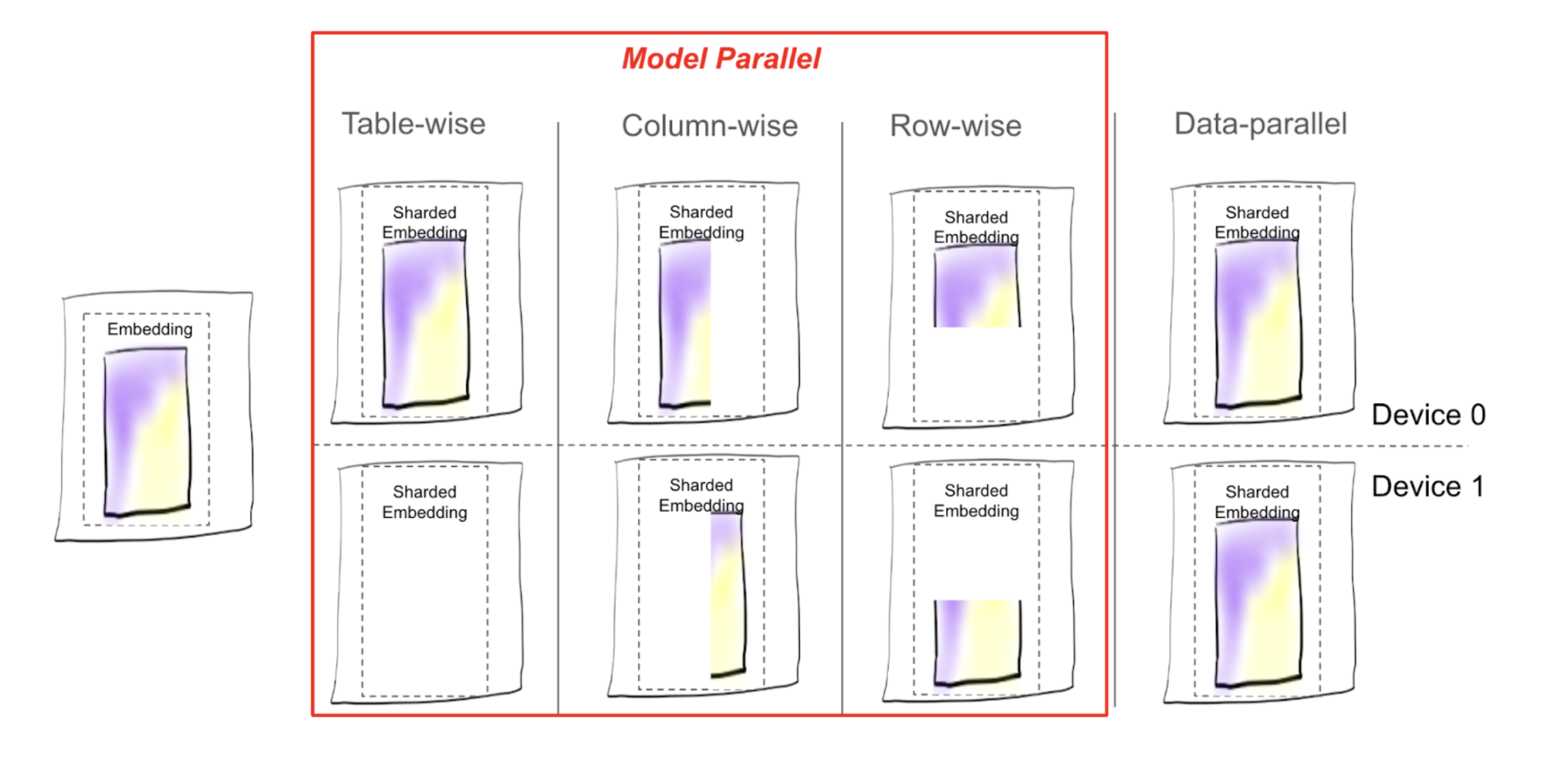
Figure 1: Visualizing the placement of table shards under different sharding schemes offered in TorchRec

Here is the list of all sharding types available in TorchRec:

• Table-wise (TW): as the name suggests, embedding table is kept as a whole piece and placed on one rank.

• Column-wise (CW): the table is split along the emb_dim dimension, for example, emb_dim=256 is split into 4 shards: [64, 64, 64, 64].

• Row-wise (RW): the table is split along the hash_size dimension, usually split evenly among all the ranks.

• Table-wise-row-wise (TWRW): table is placed on one host, split row-wise among the ranks on that host.

• Grid-shard (GS): a table is CW sharded and each CW shard is placed TWRW on a host.

• Data parallel (DP): each rank keeps a copy of the table.

Once sharded, the modules are converted to sharded versions of themselves, known as ShardedEmbeddingCollection and ShardedEmbeddingBagCollection in TorchRec. These modules handle the communication of input data, embedding lookups, and gradients.

Distributed Training with TorchRec Sharded Modules

With many sharding strategies available, how do we determine which one to use? There is a cost associated with each sharding scheme, which in conjunction with model size and number of GPUs determines which sharding strategy is best for a model.

Without sharding, where each GPU keeps a copy of the embedding table (DP), the main cost is computation in which each GPU looks up the embedding vectors in its memory in the forward pass and updates the gradients in the backward pass.

With sharding, there is an added communication cost: each GPU needs to ask the other GPUs for embedding vector lookup and communicate the gradients computed as well. This is typically referred to as all2all communication. In TorchRec, for input data on a given GPU, we determine where the embedding shard for each part of the data is located and send it to the target GPU. That target GPU then returns the embedding vectors back to the original GPU. In the backward pass, the gradients are sent back to the target GPU and the shards are updated accordingly with the optimizer.

As described above, sharding requires us to communicate the input data and embedding lookups. TorchRec handles this in three main stages, we will refer to this as the sharded embedding module forward that is used in training and inference of a TorchRec model:

• Feature All to All/Input distribution (input_dist)

  • Communicate input data (in the form of a KeyedJaggedTensor) to the appropriate device containing relevant embedding table shard

• Embedding Lookup

  • Lookup embeddings with new input data formed after feature all to all exchange

• Embedding All to All/Output Distribution (output_dist)

  • Communicate embedding lookup data back to the appropriate device that asked for it (in accordance with the input data the device received)

• The backward pass does the same operations but in reverse order.

The diagram below demonstrates how it works:

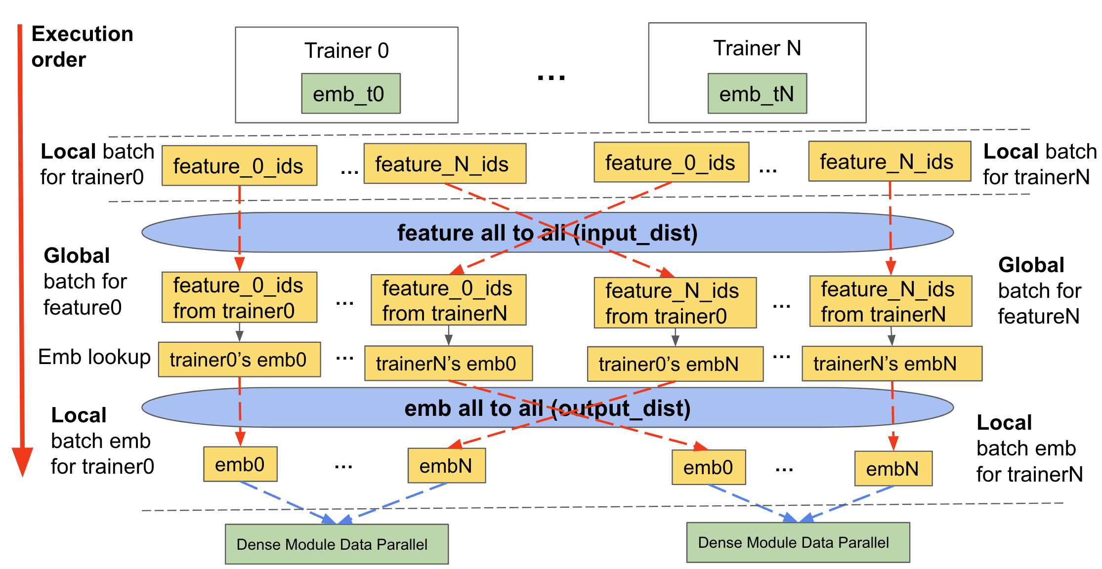
Figure 2: Forward pass of a table wise sharded table including the input_dist, lookup, and output_dist of a sharded TorchRec module

DistributedModelParallel

All of the above culminates into the main entrypoint that TorchRec uses to shard and integrate the plan. At a high level, DistributedModelParallel does the following:

• Initializes the environment by setting up process groups and assigning device type.

• Uses default shaders if no shaders are provided, the default includes EmbeddingBagCollectionSharder.

• Takes in the provided sharding plan, if none is provided, it generates one.

• Creates a sharded version of modules and replaces the original modules with them, for example, converts EmbeddingCollection to ShardedEmbeddingCollection.

• By default, wraps the DistributedModelParallel with DistributedDataParallel to make the module both model and data parallel.

Optimizer

TorchRec modules provide a seamless API to fuse the backwards pass and optimizer step in training, providing a significant optimization in performance and decreasing the memory used, alongside granularity in assigning distinct optimizers to distinct model parameters.

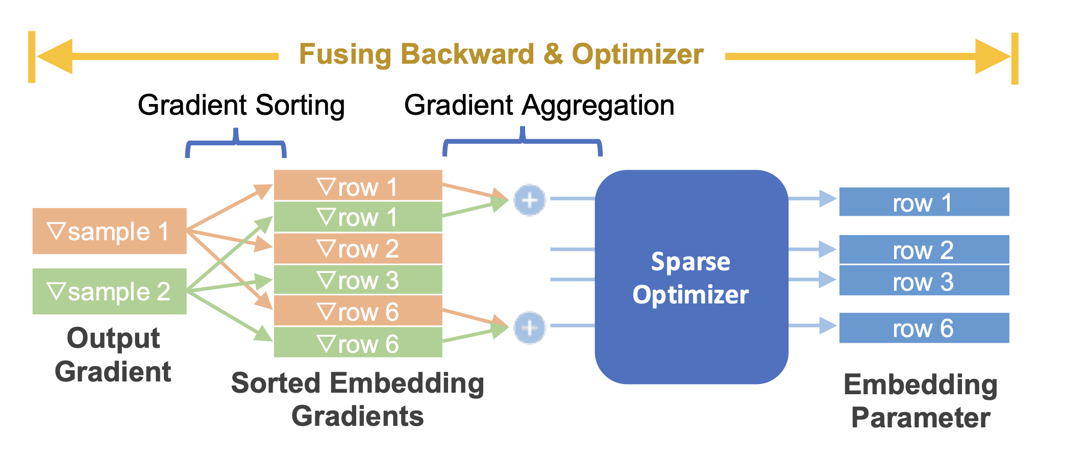
Figure 3: Fusing embedding backward with sparse optimizer

Inference

Inference environments are different from training, they are very sensitive to performance and the size of the model. There are two key differences TorchRec inference optimizes for:

• Quantization: inference models are quantized for lower latency and reduced model size. This optimization lets us use as few devices as possible for inference to minimize latency.

• C++ environment: to minimize latency even further, the model is ran in a C++ environment.

TorchRec provides the following to convert a TorchRec model into being inference ready:

• APIs for quantizing the model, including optimizations automatically with FBGEMM TBE

• Sharding embeddings for distributed inference

• Compiling the model to TorchScript (compatible in C++)

See Also

• TorchRec Interactive Notebook using the concepts