Music Source Separation with Hybrid Demucs

Author: Sean Kim

This tutorial shows how to use the Hybrid Demucs model in order to perform music separation

1. Overview

Performing music separation is composed of the following steps

1. Build the Hybrid Demucs pipeline.

2. Format the waveform into chunks of expected sizes and loop through chunks (with overlap) and feed into pipeline.

3. Collect output chunks and combine according to the way they have been overlapped.

The Hybrid Demucs [Défossez, 2021] model is a developed version of the Demucs model, a waveform based model which separates music into its respective sources, such as vocals, bass, and drums. Hybrid Demucs effectively uses spectrogram to learn through the frequency domain and also moves to time convolutions.

2. Preparation

First, we install the necessary dependencies. The first requirement is torchaudio and torch

import torch
import torchaudio

print(torch.__version__)
print(torchaudio.__version__)

1.13.0
0.13.0

In addition to torchaudio, mir_eval is required to perform signal-to-distortion ratio (SDR) calculations. To install mir_eval please use pip3 install mir_eval.

from IPython.display import Audio
from torchaudio.utils import download_asset
import matplotlib.pyplot as plt

try:
    from torchaudio.pipelines import HDEMUCS_HIGH_MUSDB_PLUS
    from mir_eval import separation

except ModuleNotFoundError:
    try:
        import google.colab

        print(
            """
            To enable running this notebook in Google Colab, install nightly
            torch and torchaudio builds by adding the following code block to the top
            of the notebook before running it:
            !pip3 uninstall -y torch torchvision torchaudio
            !pip3 install --pre torch torchvision torchaudio --extra-index-url https://download.pytorch.org/whl/nightly/cpu
            !pip3 install mir_eval
            """
        )
    except ModuleNotFoundError:
        pass
    raise

3. Construct the pipeline

Pre-trained model weights and related pipeline components are bundled as torchaudio.pipelines.HDEMUCS_HIGH_MUSDB_PLUS(). This is a torchaudio.models.HDemucs model trained on MUSDB18-HQ and additional internal extra training data. This specific model is suited for higher sample rates, around 44.1 kHZ and has a nfft value of 4096 with a depth of 6 in the model implementation.

bundle = HDEMUCS_HIGH_MUSDB_PLUS

model = bundle.get_model()

device = torch.device("cuda:0" if torch.cuda.is_available() else "cpu")

model.to(device)

sample_rate = bundle.sample_rate

print(f"Sample rate: {sample_rate}")

  0%|          | 0.00/319M [00:00<?, ?B/s]
 12%|#2        | 39.2M/319M [00:00<00:00, 411MB/s]
 25%|##5       | 80.8M/319M [00:00<00:00, 426MB/s]
 38%|###8      | 122M/319M [00:00<00:00, 428MB/s]
 51%|#####1    | 164M/319M [00:00<00:00, 432MB/s]
 64%|######4   | 205M/319M [00:00<00:00, 432MB/s]
 77%|#######7  | 247M/319M [00:00<00:00, 434MB/s]
 90%|######### | 288M/319M [00:00<00:00, 434MB/s]
100%|##########| 319M/319M [00:00<00:00, 430MB/s]
Sample rate: 44100

4. Configure the application function

Because HDemucs is a large and memory-consuming model it is very difficult to have sufficient memory to apply the model to an entire song at once. To work around this limitation, obtain the separated sources of a full song by chunking the song into smaller segments and run through the model piece by piece, and then rearrange back together.

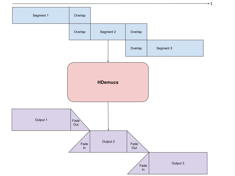
When doing this, it is important to ensure some overlap between each of the chunks, to accommodate for artifacts at the edges. Due to the nature of the model, sometimes the edges have inaccurate or undesired sounds included.

We provide a sample implementation of chunking and arrangement below. This implementation takes an overlap of 1 second on each side, and then does a linear fade in and fade out on each side. Using the faded overlaps, I add these segments together, to ensure a constant volume throughout. This accommodates for the artifacts by using less of the edges of the model outputs.

from torchaudio.transforms import Fade


def separate_sources(
        model,
        mix,
        segment=10.,
        overlap=0.1,
        device=None,
):
    """
    Apply model to a given mixture. Use fade, and add segments together in order to add model segment by segment.

    Args:
        segment (int): segment length in seconds
        device (torch.device, str, or None): if provided, device on which to
            execute the computation, otherwise `mix.device` is assumed.
            When `device` is different from `mix.device`, only local computations will
            be on `device`, while the entire tracks will be stored on `mix.device`.
    """
    if device is None:
        device = mix.device
    else:
        device = torch.device(device)

    batch, channels, length = mix.shape

    chunk_len = int(sample_rate * segment * (1 + overlap))
    start = 0
    end = chunk_len
    overlap_frames = overlap * sample_rate
    fade = Fade(fade_in_len=0, fade_out_len=int(overlap_frames), fade_shape='linear')

    final = torch.zeros(batch, len(model.sources), channels, length, device=device)

    while start < length - overlap_frames:
        chunk = mix[:, :, start:end]
        with torch.no_grad():
            out = model.forward(chunk)
        out = fade(out)
        final[:, :, :, start:end] += out
        if start == 0:
            fade.fade_in_len = int(overlap_frames)
            start += int(chunk_len - overlap_frames)
        else:
            start += chunk_len
        end += chunk_len
        if end >= length:
            fade.fade_out_len = 0
    return final


def plot_spectrogram(stft, title="Spectrogram"):
    magnitude = stft.abs()
    spectrogram = 20 * torch.log10(magnitude + 1e-8).numpy()
    figure, axis = plt.subplots(1, 1)
    img = axis.imshow(spectrogram, cmap="viridis", vmin=-60, vmax=0, origin="lower", aspect="auto")
    figure.suptitle(title)
    plt.colorbar(img, ax=axis)
    plt.show()

5. Run Model

Finally, we run the model and store the separate source files in a directory

As a test song, we will be using A Classic Education by NightOwl from MedleyDB (Creative Commons BY-NC-SA 4.0). This is also located in MUSDB18-HQ dataset within the train sources.

In order to test with a different song, the variable names and urls below can be changed alongside with the parameters to test the song separator in different ways.

# We download the audio file from our storage. Feel free to download another file and use audio from a specific path
SAMPLE_SONG = download_asset("tutorial-assets/hdemucs_mix.wav")
waveform, sample_rate = torchaudio.load(SAMPLE_SONG)  # replace SAMPLE_SONG with desired path for different song
waveform.to(device)
mixture = waveform

# parameters
segment: int = 10
overlap = 0.1

print("Separating track")

ref = waveform.mean(0)
waveform = (waveform - ref.mean()) / ref.std()  # normalization

sources = separate_sources(
    model,
    waveform[None],
    device=device,
    segment=segment,
    overlap=overlap,
)[0]
sources = sources * ref.std() + ref.mean()

sources_list = model.sources
sources = list(sources)

audios = dict(zip(sources_list, sources))

  0%|          | 0.00/28.8M [00:00<?, ?B/s]
100%|##########| 28.8M/28.8M [00:00<00:00, 420MB/s]
Separating track

5.1 Separate Track

The default set of pretrained weights that has been loaded has 4 sources that it is separated into: drums, bass, other, and vocals in that order. They have been stored into the dict “audios” and therefore can be accessed there. For the four sources, there is a separate cell for each, that will create the audio, the spectrogram graph, and also calculate the SDR score. SDR is the signal-to-distortion ratio, essentially a representation to the “quality” of an audio track.

N_FFT = 4096
N_HOP = 4
stft = torchaudio.transforms.Spectrogram(
    n_fft=N_FFT,
    hop_length=N_HOP,
    power=None,
)

5.2 Audio Segmenting and Processing

Below is the processing steps and segmenting 5 seconds of the tracks in order to feed into the spectrogram and to caclulate the respective SDR scores.

def output_results(original_source: torch.Tensor, predicted_source: torch.Tensor, source: str):
    print("SDR score is:",
          separation.bss_eval_sources(
              original_source.detach().numpy(),
              predicted_source.detach().numpy())[0].mean())
    plot_spectrogram(stft(predicted_source)[0], f'Spectrogram {source}')
    return Audio(predicted_source, rate=sample_rate)


segment_start = 150
segment_end = 155

frame_start = segment_start * sample_rate
frame_end = segment_end * sample_rate

drums_original = download_asset("tutorial-assets/hdemucs_drums_segment.wav")
bass_original = download_asset("tutorial-assets/hdemucs_bass_segment.wav")
vocals_original = download_asset("tutorial-assets/hdemucs_vocals_segment.wav")
other_original = download_asset("tutorial-assets/hdemucs_other_segment.wav")

drums_spec = audios["drums"][:, frame_start: frame_end]
drums, sample_rate = torchaudio.load(drums_original)
drums.to(device)

bass_spec = audios["bass"][:, frame_start: frame_end]
bass, sample_rate = torchaudio.load(bass_original)
bass.to(device)

vocals_spec = audios["vocals"][:, frame_start: frame_end]
vocals, sample_rate = torchaudio.load(vocals_original)
vocals.to(device)

other_spec = audios["other"][:, frame_start: frame_end]
other, sample_rate = torchaudio.load(other_original)
other.to(device)

mix_spec = mixture[:, frame_start: frame_end]

  0%|          | 0.00/1.68M [00:00<?, ?B/s]
100%|##########| 1.68M/1.68M [00:00<00:00, 217MB/s]

  0%|          | 0.00/1.68M [00:00<?, ?B/s]
100%|##########| 1.68M/1.68M [00:00<00:00, 166MB/s]

  0%|          | 0.00/1.68M [00:00<?, ?B/s]
100%|##########| 1.68M/1.68M [00:00<00:00, 217MB/s]

  0%|          | 0.00/1.68M [00:00<?, ?B/s]
100%|##########| 1.68M/1.68M [00:00<00:00, 70.5MB/s]

5.3 Spectrograms and Audio

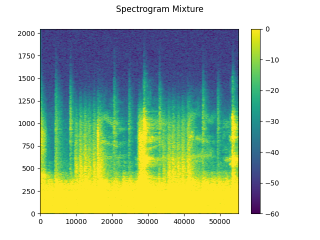
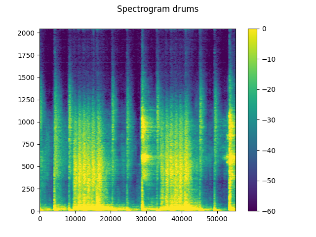
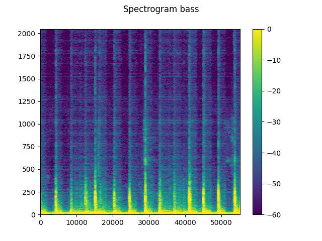
In the next 5 cells, you can see the spectrograms with the respective audios. The audios can be clearly visualized using the spectrogram.

The mixture clip comes from the original track, and the remaining tracks are the model output

# Mixture Clip
plot_spectrogram(stft(mix_spec)[0], "Spectrogram Mixture")
Audio(mix_spec, rate=sample_rate)

Drums SDR, Spectrogram, and Audio

# Drums Clip
output_results(drums, drums_spec, "drums")

SDR score is: 5.0177358299400145

Bass SDR, Spectrogram, and Audio

# Bass Clip
output_results(bass, bass_spec, "bass")

SDR score is: 18.90925258121451

Vocals SDR, Spectrogram, and Audio

# Vocals Audio
output_results(vocals, vocals_spec, "vocals")

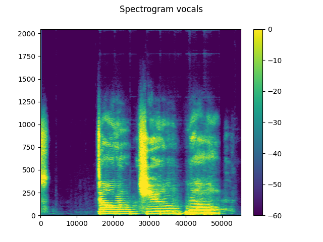
SDR score is: 8.792411080980822

Other SDR, Spectrogram, and Audio

# Other Clip
output_results(other, other_spec, "other")

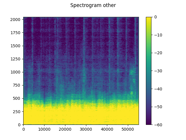
SDR score is: 8.868967320016406

# Optionally, the full audios can be heard in from running the next 5
# cells. They will take a bit longer to load, so to run simply uncomment
# out the ``Audio`` cells for the respective track to produce the audio
# for the full song.
#

# Full Audio
# Audio(mixture, rate=sample_rate)

# Drums Audio
# Audio(audios["drums"], rate=sample_rate)

# Bass Audio
# Audio(audios["bass"], rate=sample_rate)

# Vocals Audio
# Audio(audios["vocals"], rate=sample_rate)

# Other Audio
# Audio(audios["other"], rate=sample_rate)