Speech Enhancement with MVDR Beamforming

Author Zhaoheng Ni

1. Overview

This is a tutorial on applying Minimum Variance Distortionless Response (MVDR) beamforming to estimate enhanced speech with TorchAudio.

Steps:

• Generate an ideal ratio mask (IRM) by dividing the clean/noise magnitude by the mixture magnitude.

• Estimate power spectral density (PSD) matrices using torchaudio.transforms.PSD().

• Estimate enhanced speech using MVDR modules (torchaudio.transforms.SoudenMVDR() and torchaudio.transforms.RTFMVDR()).

• Benchmark the two methods (torchaudio.functional.rtf_evd() and torchaudio.functional.rtf_power()) for computing the relative transfer function (RTF) matrix of the reference microphone.

import torch
import torchaudio
import torchaudio.functional as F

print(torch.__version__)
print(torchaudio.__version__)

Out:

1.12.0
0.12.0

2. Preparation

First, we import the necessary packages and retrieve the data.

The multi-channel audio example is selected from ConferencingSpeech dataset.

The original filename is

SSB07200001\#noise-sound-bible-0038\#7.86_6.16_3.00_3.14_4.84_134.5285_191.7899_0.4735\#15217\#25.16333303751458\#0.2101221178590021.wav

which was generated with:

• SSB07200001.wav from AISHELL-3 (Apache License v.2.0)

• noise-sound-bible-0038.wav from MUSAN (Attribution 4.0 International — CC BY 4.0)

import matplotlib.pyplot as plt
from IPython.display import Audio
from torchaudio.utils import download_asset

SAMPLE_RATE = 16000
SAMPLE_CLEAN = download_asset("tutorial-assets/mvdr/clean_speech.wav")
SAMPLE_NOISE = download_asset("tutorial-assets/mvdr/noise.wav")

Out:

  0%|          | 0.00/0.98M [00:00<?, ?B/s]
100%|##########| 0.98M/0.98M [00:00<00:00, 81.9MB/s]

  0%|          | 0.00/1.95M [00:00<?, ?B/s]
100%|##########| 1.95M/1.95M [00:00<00:00, 44.2MB/s]

2.1. Helper functions

def plot_spectrogram(stft, title="Spectrogram", xlim=None):
    magnitude = stft.abs()
    spectrogram = 20 * torch.log10(magnitude + 1e-8).numpy()
    figure, axis = plt.subplots(1, 1)
    img = axis.imshow(spectrogram, cmap="viridis", vmin=-100, vmax=0, origin="lower", aspect="auto")
    figure.suptitle(title)
    plt.colorbar(img, ax=axis)
    plt.show()


def plot_mask(mask, title="Mask", xlim=None):
    mask = mask.numpy()
    figure, axis = plt.subplots(1, 1)
    img = axis.imshow(mask, cmap="viridis", origin="lower", aspect="auto")
    figure.suptitle(title)
    plt.colorbar(img, ax=axis)
    plt.show()


def si_snr(estimate, reference, epsilon=1e-8):
    estimate = estimate - estimate.mean()
    reference = reference - reference.mean()
    reference_pow = reference.pow(2).mean(axis=1, keepdim=True)
    mix_pow = (estimate * reference).mean(axis=1, keepdim=True)
    scale = mix_pow / (reference_pow + epsilon)

    reference = scale * reference
    error = estimate - reference

    reference_pow = reference.pow(2)
    error_pow = error.pow(2)

    reference_pow = reference_pow.mean(axis=1)
    error_pow = error_pow.mean(axis=1)

    si_snr = 10 * torch.log10(reference_pow) - 10 * torch.log10(error_pow)
    return si_snr.item()

3. Generate Ideal Ratio Masks (IRMs)

3.1. Load audio data

waveform_clean, sr = torchaudio.load(SAMPLE_CLEAN)
waveform_noise, sr2 = torchaudio.load(SAMPLE_NOISE)
assert sr == sr2 == SAMPLE_RATE
# The mixture waveform is a combination of clean and noise waveforms
waveform_mix = waveform_clean + waveform_noise

Note: To improve computational robustness, it is recommended to represent the waveforms as double-precision floating point (torch.float64 or torch.double) values.

waveform_mix = waveform_mix.to(torch.double)
waveform_clean = waveform_clean.to(torch.double)
waveform_noise = waveform_noise.to(torch.double)

3.2. Compute STFT coefficients

N_FFT = 1024
N_HOP = 256
stft = torchaudio.transforms.Spectrogram(
    n_fft=N_FFT,
    hop_length=N_HOP,
    power=None,
)
istft = torchaudio.transforms.InverseSpectrogram(n_fft=N_FFT, hop_length=N_HOP)

stft_mix = stft(waveform_mix)
stft_clean = stft(waveform_clean)
stft_noise = stft(waveform_noise)

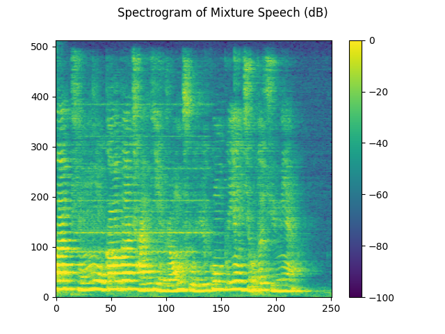
3.2.1. Visualize mixture speech

plot_spectrogram(stft_mix[0], "Spectrogram of Mixture Speech (dB)")
Audio(waveform_mix[0], rate=SAMPLE_RATE)

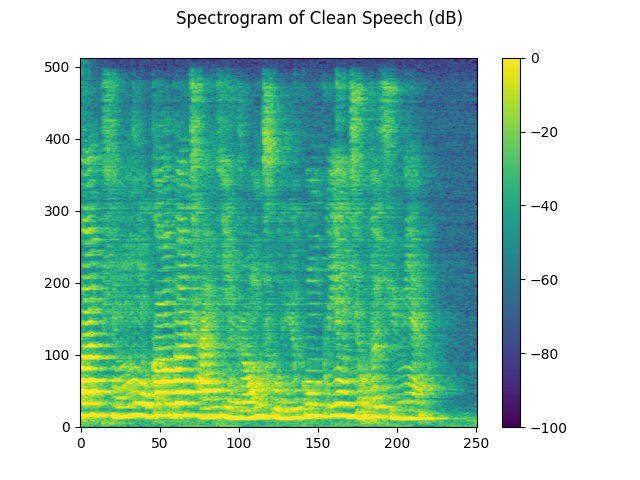
3.2.2. Visualize clean speech

plot_spectrogram(stft_clean[0], "Spectrogram of Clean Speech (dB)")
Audio(waveform_clean[0], rate=SAMPLE_RATE)

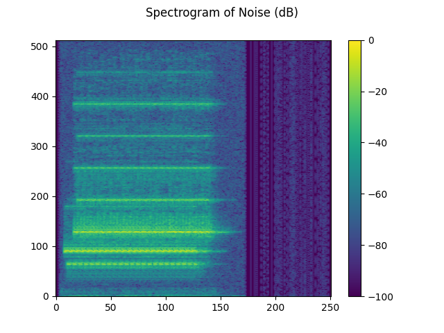
3.2.3. Visualize noise

plot_spectrogram(stft_noise[0], "Spectrogram of Noise (dB)")
Audio(waveform_noise[0], rate=SAMPLE_RATE)

3.3. Define the reference microphone

We choose the first microphone in the array as the reference channel for demonstration. The selection of the reference channel may depend on the design of the microphone array.

You can also apply an end-to-end neural network which estimates both the reference channel and the PSD matrices, then obtains the enhanced STFT coefficients by the MVDR module.

REFERENCE_CHANNEL = 0

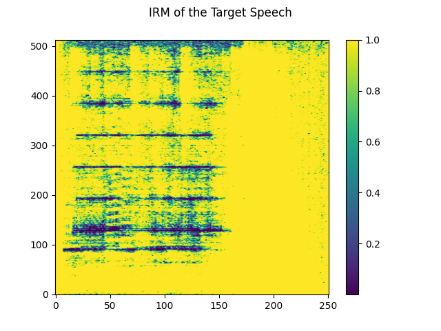
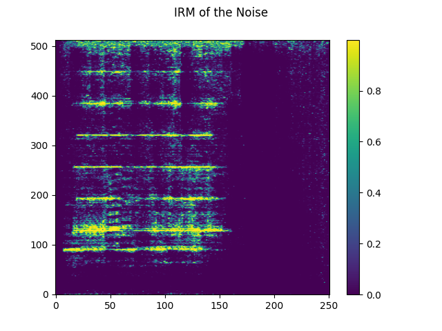
3.4. Compute IRMs

def get_irms(stft_clean, stft_noise):
    mag_clean = stft_clean.abs() ** 2
    mag_noise = stft_noise.abs() ** 2
    irm_speech = mag_clean / (mag_clean + mag_noise)
    irm_noise = mag_noise / (mag_clean + mag_noise)
    return irm_speech[REFERENCE_CHANNEL], irm_noise[REFERENCE_CHANNEL]


irm_speech, irm_noise = get_irms(stft_clean, stft_noise)

3.4.1. Visualize IRM of target speech

plot_mask(irm_speech, "IRM of the Target Speech")

3.4.2. Visualize IRM of noise

plot_mask(irm_noise, "IRM of the Noise")

4. Compute PSD matrices

torchaudio.transforms.PSD() computes the time-invariant PSD matrix given the multi-channel complex-valued STFT coefficients of the mixture speech and the time-frequency mask.

The shape of the PSD matrix is (…, freq, channel, channel).

psd_transform = torchaudio.transforms.PSD()

psd_speech = psd_transform(stft_mix, irm_speech)
psd_noise = psd_transform(stft_mix, irm_noise)

5. Beamforming using SoudenMVDR

5.1. Apply beamforming

torchaudio.transforms.SoudenMVDR() takes the multi-channel complexed-valued STFT coefficients of the mixture speech, PSD matrices of target speech and noise, and the reference channel inputs.

The output is a single-channel complex-valued STFT coefficients of the enhanced speech. We can then obtain the enhanced waveform by passing this output to the torchaudio.transforms.InverseSpectrogram() module.

mvdr_transform = torchaudio.transforms.SoudenMVDR()
stft_souden = mvdr_transform(stft_mix, psd_speech, psd_noise, reference_channel=REFERENCE_CHANNEL)
waveform_souden = istft(stft_souden, length=waveform_mix.shape[-1])

5.2. Result for SoudenMVDR

plot_spectrogram(stft_souden, "Enhanced Spectrogram by SoudenMVDR (dB)")
waveform_souden = waveform_souden.reshape(1, -1)
print(f"Si-SNR score: {si_snr(waveform_souden, waveform_clean[0:1])}")
Audio(waveform_souden, rate=SAMPLE_RATE)

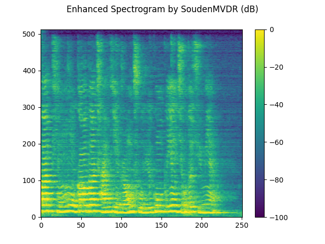
Out:

Si-SNR score: 15.035907456979267

6. Beamforming using RTFMVDR

6.1. Compute RTF

TorchAudio offers two methods for computing the RTF matrix of a target speech:

• torchaudio.functional.rtf_evd(), which applies eigenvalue decomposition to the PSD matrix of target speech to get the RTF matrix.

• torchaudio.functional.rtf_power(), which applies the power iteration method. You can specify the number of iterations with argument n_iter.

rtf_evd = F.rtf_evd(psd_speech)
rtf_power = F.rtf_power(psd_speech, psd_noise, reference_channel=REFERENCE_CHANNEL)

6.2. Apply beamforming

torchaudio.transforms.RTFMVDR() takes the multi-channel complexed-valued STFT coefficients of the mixture speech, RTF matrix of target speech, PSD matrix of noise, and the reference channel inputs.

The output is a single-channel complex-valued STFT coefficients of the enhanced speech. We can then obtain the enhanced waveform by passing this output to the torchaudio.transforms.InverseSpectrogram() module.

mvdr_transform = torchaudio.transforms.RTFMVDR()

# compute the enhanced speech based on F.rtf_evd
stft_rtf_evd = mvdr_transform(stft_mix, rtf_evd, psd_noise, reference_channel=REFERENCE_CHANNEL)
waveform_rtf_evd = istft(stft_rtf_evd, length=waveform_mix.shape[-1])

# compute the enhanced speech based on F.rtf_power
stft_rtf_power = mvdr_transform(stft_mix, rtf_power, psd_noise, reference_channel=REFERENCE_CHANNEL)
waveform_rtf_power = istft(stft_rtf_power, length=waveform_mix.shape[-1])

6.3. Result for RTFMVDR with rtf_evd

plot_spectrogram(stft_rtf_evd, "Enhanced Spectrogram by RTFMVDR and F.rtf_evd (dB)")
waveform_rtf_evd = waveform_rtf_evd.reshape(1, -1)
print(f"Si-SNR score: {si_snr(waveform_rtf_evd, waveform_clean[0:1])}")
Audio(waveform_rtf_evd, rate=SAMPLE_RATE)

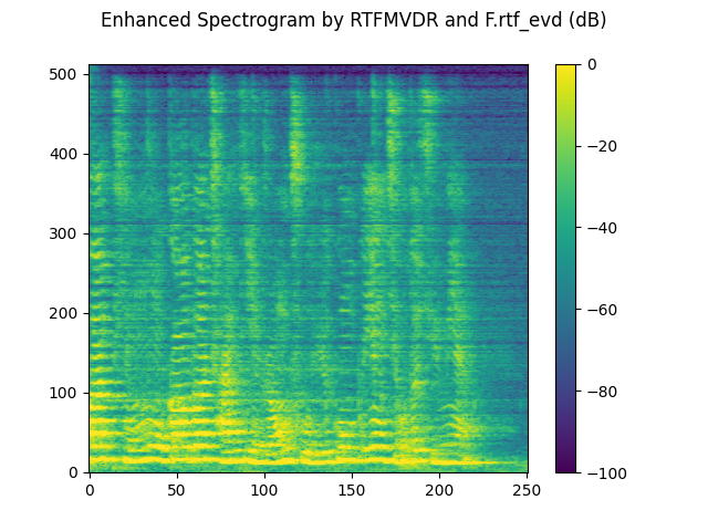
Out:

Si-SNR score: 16.563734673832403

6.4. Result for RTFMVDR with rtf_power

plot_spectrogram(stft_rtf_power, "Enhanced Spectrogram by RTFMVDR and F.rtf_evd (dB)")
waveform_rtf_power = waveform_rtf_power.reshape(1, -1)
print(f"Si-SNR score: {si_snr(waveform_rtf_power, waveform_clean[0:1])}")
Audio(waveform_rtf_power, rate=SAMPLE_RATE)

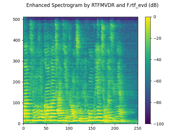
Out:

Si-SNR score: 17.820481909930376