Audio Data Augmentation

torchaudio provides a variety of ways to augment audio data.

In this tutorial, we look into a way to apply effects, filters, RIR (room impulse response) and codecs.

At the end, we synthesize noisy speech over phone from clean speech.

import torch
import torchaudio
import torchaudio.functional as F

print(torch.__version__)
print(torchaudio.__version__)

Out:

1.12.0
0.12.0

Preparation

First, we import the modules and download the audio assets we use in this tutorial.

import math

from IPython.display import Audio
import matplotlib.pyplot as plt

from torchaudio.utils import download_asset

SAMPLE_WAV = download_asset("tutorial-assets/steam-train-whistle-daniel_simon.wav")
SAMPLE_RIR = download_asset("tutorial-assets/Lab41-SRI-VOiCES-rm1-impulse-mc01-stu-clo-8000hz.wav")
SAMPLE_SPEECH = download_asset("tutorial-assets/Lab41-SRI-VOiCES-src-sp0307-ch127535-sg0042-8000hz.wav")
SAMPLE_NOISE = download_asset("tutorial-assets/Lab41-SRI-VOiCES-rm1-babb-mc01-stu-clo-8000hz.wav")

Out:

  0%|          | 0.00/427k [00:00<?, ?B/s]
100%|##########| 427k/427k [00:00<00:00, 67.1MB/s]

  0%|          | 0.00/31.3k [00:00<?, ?B/s]
100%|##########| 31.3k/31.3k [00:00<00:00, 11.5MB/s]

  0%|          | 0.00/78.2k [00:00<?, ?B/s]
100%|##########| 78.2k/78.2k [00:00<00:00, 20.9MB/s]

Applying effects and filtering

torchaudio.sox_effects() allows for directly applying filters similar to those available in sox to Tensor objects and file object audio sources.

There are two functions for this:

• torchaudio.sox_effects.apply_effects_tensor() for applying effects to Tensor.

• torchaudio.sox_effects.apply_effects_file() for applying effects to other audio sources.

Both functions accept effect definitions in the form List[List[str]]. This is mostly consistent with how sox command works, but one caveat is that sox adds some effects automatically, whereas torchaudio’s implementation does not.

For the list of available effects, please refer to the sox documentation.

Tip If you need to load and resample your audio data on the fly, then you can use torchaudio.sox_effects.apply_effects_file() with effect "rate".

Note torchaudio.sox_effects.apply_effects_file() accepts a file-like object or path-like object. Similar to torchaudio.load(), when the audio format cannot be inferred from either the file extension or header, you can provide argument format to specify the format of the audio source.

Note This process is not differentiable.

# Load the data
waveform1, sample_rate1 = torchaudio.load(SAMPLE_WAV)

# Define effects
effects = [
    ["lowpass", "-1", "300"],  # apply single-pole lowpass filter
    ["speed", "0.8"],  # reduce the speed
    # This only changes sample rate, so it is necessary to
    # add `rate` effect with original sample rate after this.
    ["rate", f"{sample_rate1}"],
    ["reverb", "-w"],  # Reverbration gives some dramatic feeling
]

# Apply effects
waveform2, sample_rate2 = torchaudio.sox_effects.apply_effects_tensor(waveform1, sample_rate1, effects)

print(waveform1.shape, sample_rate1)
print(waveform2.shape, sample_rate2)

Out:

torch.Size([2, 109368]) 44100
torch.Size([2, 136710]) 44100

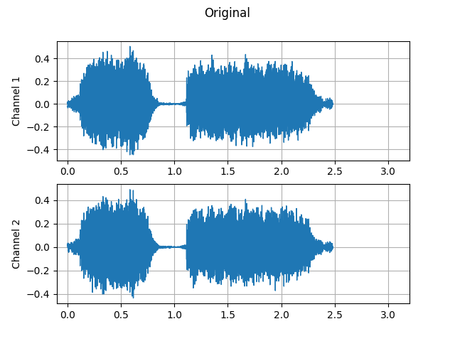
Note that the number of frames and number of channels are different from those of the original after the effects are applied. Let’s listen to the audio.

def plot_waveform(waveform, sample_rate, title="Waveform", xlim=None):
    waveform = waveform.numpy()

    num_channels, num_frames = waveform.shape
    time_axis = torch.arange(0, num_frames) / sample_rate

    figure, axes = plt.subplots(num_channels, 1)
    if num_channels == 1:
        axes = [axes]
    for c in range(num_channels):
        axes[c].plot(time_axis, waveform[c], linewidth=1)
        axes[c].grid(True)
        if num_channels > 1:
            axes[c].set_ylabel(f"Channel {c+1}")
        if xlim:
            axes[c].set_xlim(xlim)
    figure.suptitle(title)
    plt.show(block=False)

def plot_specgram(waveform, sample_rate, title="Spectrogram", xlim=None):
    waveform = waveform.numpy()

    num_channels, _ = waveform.shape

    figure, axes = plt.subplots(num_channels, 1)
    if num_channels == 1:
        axes = [axes]
    for c in range(num_channels):
        axes[c].specgram(waveform[c], Fs=sample_rate)
        if num_channels > 1:
            axes[c].set_ylabel(f"Channel {c+1}")
        if xlim:
            axes[c].set_xlim(xlim)
    figure.suptitle(title)
    plt.show(block=False)

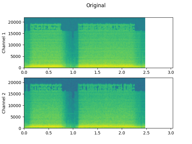
Original:

plot_waveform(waveform1, sample_rate1, title="Original", xlim=(-0.1, 3.2))
plot_specgram(waveform1, sample_rate1, title="Original", xlim=(0, 3.04))
Audio(waveform1, rate=sample_rate1)

• 
• 

Effects applied:

plot_waveform(waveform2, sample_rate2, title="Effects Applied", xlim=(-0.1, 3.2))
plot_specgram(waveform2, sample_rate2, title="Effects Applied", xlim=(0, 3.04))
Audio(waveform2, rate=sample_rate2)

• 
• 

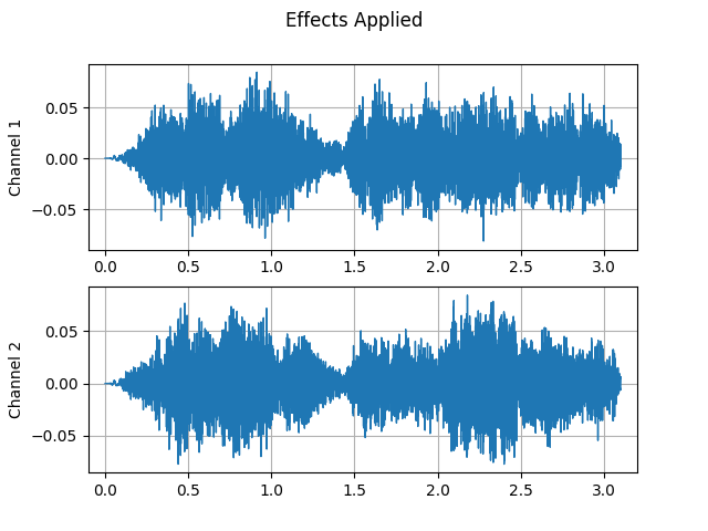
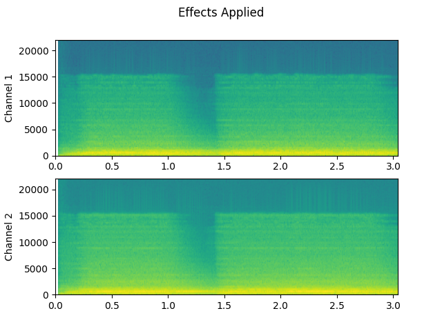
Doesn’t it sound more dramatic?

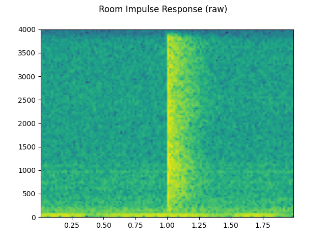
Simulating room reverberation

Convolution reverb is a technique that’s used to make clean audio sound as though it has been produced in a different environment.

Using Room Impulse Response (RIR), for instance, we can make clean speech sound as though it has been uttered in a conference room.

For this process, we need RIR data. The following data are from the VOiCES dataset, but you can record your own — just turn on your microphone and clap your hands.

rir_raw, sample_rate = torchaudio.load(SAMPLE_RIR)
plot_waveform(rir_raw, sample_rate, title="Room Impulse Response (raw)")
plot_specgram(rir_raw, sample_rate, title="Room Impulse Response (raw)")
Audio(rir_raw, rate=sample_rate)

• 
• 

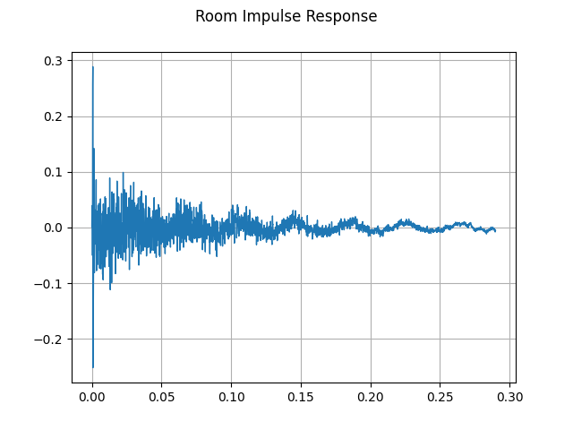
First, we need to clean up the RIR. We extract the main impulse, normalize the signal power, then flip along the time axis.

rir = rir_raw[:, int(sample_rate * 1.01) : int(sample_rate * 1.3)]
rir = rir / torch.norm(rir, p=2)
RIR = torch.flip(rir, [1])

plot_waveform(rir, sample_rate, title="Room Impulse Response")

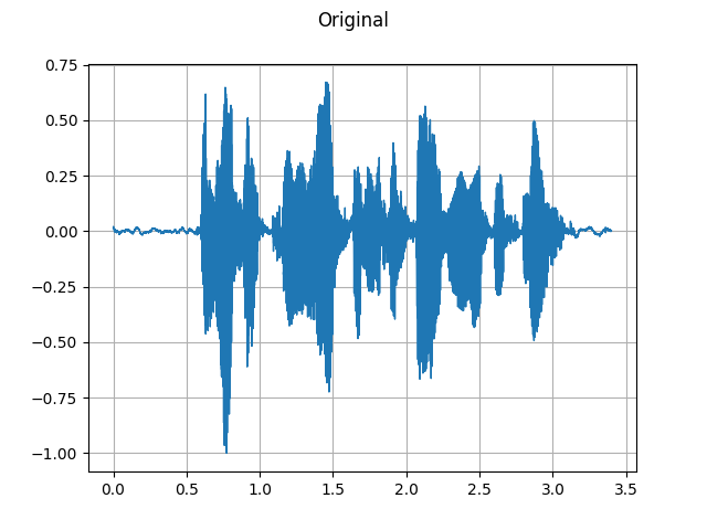
Then, we convolve the speech signal with the RIR filter.

speech, _ = torchaudio.load(SAMPLE_SPEECH)

speech_ = torch.nn.functional.pad(speech, (RIR.shape[1] - 1, 0))
augmented = torch.nn.functional.conv1d(speech_[None, ...], RIR[None, ...])[0]

Original:

plot_waveform(speech, sample_rate, title="Original")
plot_specgram(speech, sample_rate, title="Original")
Audio(speech, rate=sample_rate)

• 
• 

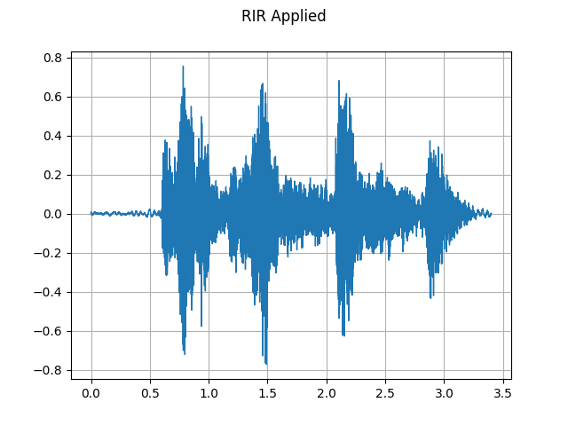
RIR applied:

plot_waveform(augmented, sample_rate, title="RIR Applied")
plot_specgram(augmented, sample_rate, title="RIR Applied")
Audio(augmented, rate=sample_rate)

• 
• 

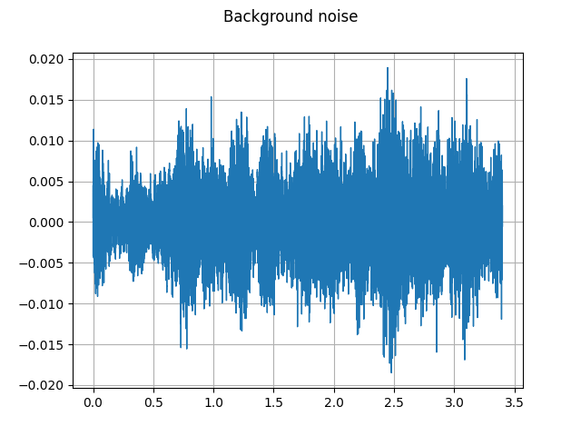
Adding background noise

To add background noise to audio data, you can simply add a noise Tensor to the Tensor representing the audio data. A common method to adjust the intensity of noise is changing the Signal-to-Noise Ratio (SNR). [wikipedia]

$$ \mathrm{SNR} = \frac{P_{signal}}{P_{noise}} $$

$$ \mathrm{SNR_{dB}} = 10 \log _{{10}} \mathrm {SNR} $$

speech, _ = torchaudio.load(SAMPLE_SPEECH)
noise, _ = torchaudio.load(SAMPLE_NOISE)
noise = noise[:, : speech.shape[1]]

speech_power = speech.norm(p=2)
noise_power = noise.norm(p=2)

snr_dbs = [20, 10, 3]
noisy_speeches = []
for snr_db in snr_dbs:
    snr = 10 ** (snr_db / 20)
    scale = snr * noise_power / speech_power
    noisy_speeches.append((scale * speech + noise) / 2)

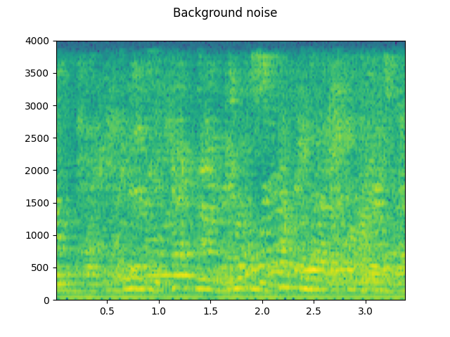
Background noise:

plot_waveform(noise, sample_rate, title="Background noise")
plot_specgram(noise, sample_rate, title="Background noise")
Audio(noise, rate=sample_rate)

• 
• 

SNR 20 dB:

snr_db, noisy_speech = snr_dbs[0], noisy_speeches[0]
plot_waveform(noisy_speech, sample_rate, title=f"SNR: {snr_db} [dB]")
plot_specgram(noisy_speech, sample_rate, title=f"SNR: {snr_db} [dB]")
Audio(noisy_speech, rate=sample_rate)

• 
• 

SNR 10 dB:

snr_db, noisy_speech = snr_dbs[1], noisy_speeches[1]
plot_waveform(noisy_speech, sample_rate, title=f"SNR: {snr_db} [dB]")
plot_specgram(noisy_speech, sample_rate, title=f"SNR: {snr_db} [dB]")
Audio(noisy_speech, rate=sample_rate)

• 
• 

SNR 3 dB:

snr_db, noisy_speech = snr_dbs[2], noisy_speeches[2]
plot_waveform(noisy_speech, sample_rate, title=f"SNR: {snr_db} [dB]")
plot_specgram(noisy_speech, sample_rate, title=f"SNR: {snr_db} [dB]")
Audio(noisy_speech, rate=sample_rate)

• 
• 

Applying codec to Tensor object

torchaudio.functional.apply_codec() can apply codecs to a Tensor object.

Note This process is not differentiable.

waveform, sample_rate = torchaudio.load(SAMPLE_SPEECH)

configs = [
    {"format": "wav", "encoding": "ULAW", "bits_per_sample": 8},
    {"format": "gsm"},
    {"format": "vorbis", "compression": -1},
]
waveforms = []
for param in configs:
    augmented = F.apply_codec(waveform, sample_rate, **param)
    waveforms.append(augmented)

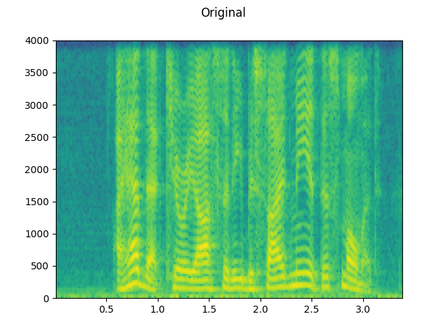
Original:

plot_waveform(waveform, sample_rate, title="Original")
plot_specgram(waveform, sample_rate, title="Original")
Audio(waveform, rate=sample_rate)

• 
• 

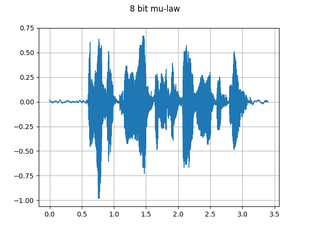
8 bit mu-law:

plot_waveform(waveforms[0], sample_rate, title="8 bit mu-law")
plot_specgram(waveforms[0], sample_rate, title="8 bit mu-law")
Audio(waveforms[0], rate=sample_rate)

• 
• 

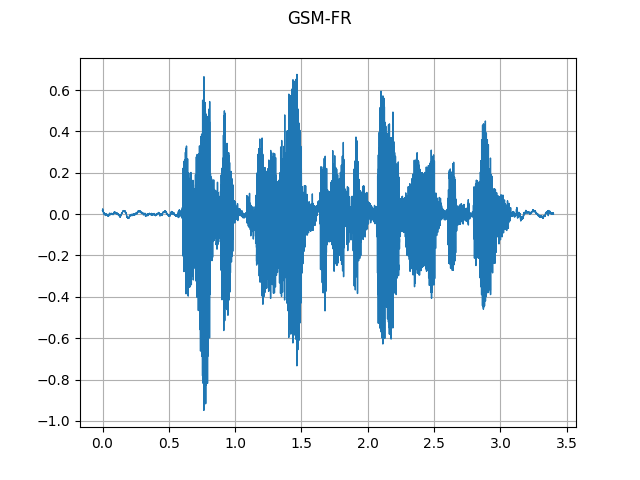
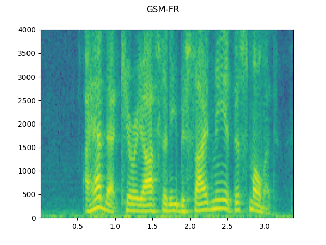
GSM-FR:

plot_waveform(waveforms[1], sample_rate, title="GSM-FR")
plot_specgram(waveforms[1], sample_rate, title="GSM-FR")
Audio(waveforms[1], rate=sample_rate)

• 
• 

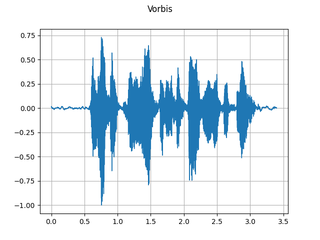
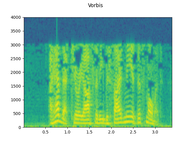
Vorbis:

plot_waveform(waveforms[2], sample_rate, title="Vorbis")
plot_specgram(waveforms[2], sample_rate, title="Vorbis")
Audio(waveforms[2], rate=sample_rate)

• 
• 

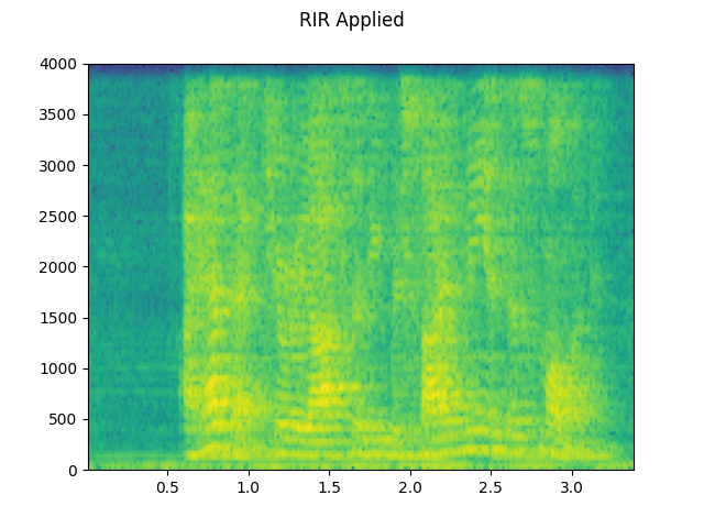
Simulating a phone recoding

Combining the previous techniques, we can simulate audio that sounds like a person talking over a phone in a echoey room with people talking in the background.

sample_rate = 16000
original_speech, sample_rate = torchaudio.load(SAMPLE_SPEECH)

plot_specgram(original_speech, sample_rate, title="Original")

# Apply RIR
speech_ = torch.nn.functional.pad(original_speech, (RIR.shape[1] - 1, 0))
rir_applied = torch.nn.functional.conv1d(speech_[None, ...], RIR[None, ...])[0]

plot_specgram(rir_applied, sample_rate, title="RIR Applied")

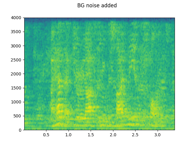
# Add background noise
# Because the noise is recorded in the actual environment, we consider that
# the noise contains the acoustic feature of the environment. Therefore, we add
# the noise after RIR application.
noise, _ = torchaudio.load(SAMPLE_NOISE)
noise = noise[:, : rir_applied.shape[1]]

snr_db = 8
scale = math.exp(snr_db / 10) * noise.norm(p=2) / rir_applied.norm(p=2)
bg_added = (scale * rir_applied + noise) / 2

plot_specgram(bg_added, sample_rate, title="BG noise added")

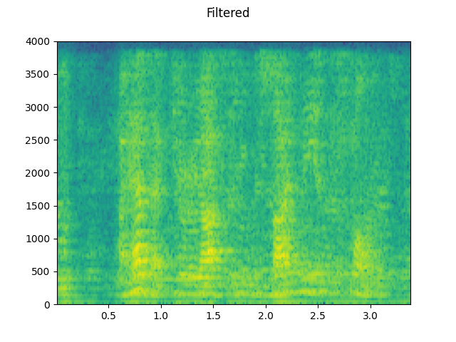
# Apply filtering and change sample rate
filtered, sample_rate2 = torchaudio.sox_effects.apply_effects_tensor(
    bg_added,
    sample_rate,
    effects=[
        ["lowpass", "4000"],
        [
            "compand",
            "0.02,0.05",
            "-60,-60,-30,-10,-20,-8,-5,-8,-2,-8",
            "-8",
            "-7",
            "0.05",
        ],
        ["rate", "8000"],
    ],
)

plot_specgram(filtered, sample_rate2, title="Filtered")

# Apply telephony codec
codec_applied = F.apply_codec(filtered, sample_rate2, format="gsm")

plot_specgram(codec_applied, sample_rate2, title="GSM Codec Applied")

• 
• 
• 
• 
• 

Original speech:

Audio(original_speech, rate=sample_rate)

RIR applied:

Audio(rir_applied, rate=sample_rate)

Background noise added:

Audio(bg_added, rate=sample_rate)

Filtered:

Audio(filtered, rate=sample_rate2)

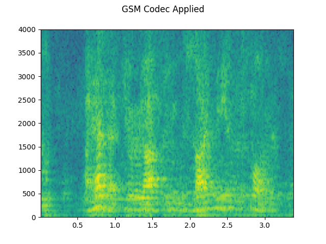
Codec aplied:

Audio(codec_applied, rate=sample_rate2)