Introduction || Tensors || Autograd || Building Models || TensorBoard Support || Training Models || Model Understanding

Training with PyTorch

Follow along with the video below or on youtube.

Introduction

In past videos, we’ve discussed and demonstrated:

• Building models with the neural network layers and functions of the torch.nn module

• The mechanics of automated gradient computation, which is central to gradient-based model training

• Using TensorBoard to visualize training progress and other activities

In this video, we’ll be adding some new tools to your inventory:

• We’ll get familiar with the dataset and dataloader abstractions, and how they ease the process of feeding data to your model during a training loop

• We’ll discuss specific loss functions and when to use them

• We’ll look at PyTorch optimizers, which implement algorithms to adjust model weights based on the outcome of a loss function

Finally, we’ll pull all of these together and see a full PyTorch training loop in action.

Dataset and DataLoader

The Dataset and DataLoader classes encapsulate the process of pulling your data from storage and exposing it to your training loop in batches.

The Dataset is responsible for accessing and processing single instances of data.

The DataLoader pulls instances of data from the Dataset (either automatically or with a sampler that you define), collects them in batches, and returns them for consumption by your training loop. The DataLoader works with all kinds of datasets, regardless of the type of data they contain.

For this tutorial, we’ll be using the Fashion-MNIST dataset provided by TorchVision. We use torchvision.transforms.Normalize() to zero-center and normalize the distribution of the image tile content, and download both training and validation data splits.

import torch
import torchvision
import torchvision.transforms as transforms

# PyTorch TensorBoard support
from torch.utils.tensorboard import SummaryWriter
from datetime import datetime


transform = transforms.Compose(
    [transforms.ToTensor(),
    transforms.Normalize((0.5,), (0.5,))])

# Create datasets for training & validation, download if necessary
training_set = torchvision.datasets.FashionMNIST('./data', train=True, transform=transform, download=True)
validation_set = torchvision.datasets.FashionMNIST('./data', train=False, transform=transform, download=True)

# Create data loaders for our datasets; shuffle for training, not for validation
training_loader = torch.utils.data.DataLoader(training_set, batch_size=4, shuffle=True)
validation_loader = torch.utils.data.DataLoader(validation_set, batch_size=4, shuffle=False)

# Class labels
classes = ('T-shirt/top', 'Trouser', 'Pullover', 'Dress', 'Coat',
        'Sandal', 'Shirt', 'Sneaker', 'Bag', 'Ankle Boot')

# Report split sizes
print('Training set has {} instances'.format(len(training_set)))
print('Validation set has {} instances'.format(len(validation_set)))

Downloading http://fashion-mnist.s3-website.eu-central-1.amazonaws.com/train-images-idx3-ubyte.gz
Downloading http://fashion-mnist.s3-website.eu-central-1.amazonaws.com/train-images-idx3-ubyte.gz to ./data/FashionMNIST/raw/train-images-idx3-ubyte.gz

  0%|          | 0/26421880 [00:00<?, ?it/s]
  0%|          | 65536/26421880 [00:00<01:12, 362925.91it/s]
  1%|          | 229376/26421880 [00:00<00:38, 682159.15it/s]
  4%|3         | 950272/26421880 [00:00<00:11, 2187081.97it/s]
 15%|#4        | 3833856/26421880 [00:00<00:02, 7607251.35it/s]
 34%|###3      | 8978432/26421880 [00:00<00:01, 15084567.00it/s]
 54%|#####4    | 14385152/26421880 [00:01<00:00, 20101263.68it/s]
 75%|#######4  | 19693568/26421880 [00:01<00:00, 23106926.53it/s]
 96%|#########6| 25427968/26421880 [00:01<00:00, 25819734.56it/s]
100%|##########| 26421880/26421880 [00:01<00:00, 18185854.56it/s]
Extracting ./data/FashionMNIST/raw/train-images-idx3-ubyte.gz to ./data/FashionMNIST/raw

Downloading http://fashion-mnist.s3-website.eu-central-1.amazonaws.com/train-labels-idx1-ubyte.gz
Downloading http://fashion-mnist.s3-website.eu-central-1.amazonaws.com/train-labels-idx1-ubyte.gz to ./data/FashionMNIST/raw/train-labels-idx1-ubyte.gz

  0%|          | 0/29515 [00:00<?, ?it/s]
100%|##########| 29515/29515 [00:00<00:00, 326013.65it/s]
Extracting ./data/FashionMNIST/raw/train-labels-idx1-ubyte.gz to ./data/FashionMNIST/raw

Downloading http://fashion-mnist.s3-website.eu-central-1.amazonaws.com/t10k-images-idx3-ubyte.gz
Downloading http://fashion-mnist.s3-website.eu-central-1.amazonaws.com/t10k-images-idx3-ubyte.gz to ./data/FashionMNIST/raw/t10k-images-idx3-ubyte.gz

  0%|          | 0/4422102 [00:00<?, ?it/s]
  1%|1         | 65536/4422102 [00:00<00:12, 359762.88it/s]
  5%|5         | 229376/4422102 [00:00<00:06, 675856.69it/s]
 17%|#7        | 753664/4422102 [00:00<00:01, 2106498.33it/s]
 39%|###8      | 1703936/4422102 [00:00<00:00, 3587620.42it/s]
100%|##########| 4422102/4422102 [00:00<00:00, 6026134.37it/s]
Extracting ./data/FashionMNIST/raw/t10k-images-idx3-ubyte.gz to ./data/FashionMNIST/raw

Downloading http://fashion-mnist.s3-website.eu-central-1.amazonaws.com/t10k-labels-idx1-ubyte.gz
Downloading http://fashion-mnist.s3-website.eu-central-1.amazonaws.com/t10k-labels-idx1-ubyte.gz to ./data/FashionMNIST/raw/t10k-labels-idx1-ubyte.gz

  0%|          | 0/5148 [00:00<?, ?it/s]
100%|##########| 5148/5148 [00:00<00:00, 42926992.03it/s]
Extracting ./data/FashionMNIST/raw/t10k-labels-idx1-ubyte.gz to ./data/FashionMNIST/raw

Training set has 60000 instances
Validation set has 10000 instances

As always, let’s visualize the data as a sanity check:

import matplotlib.pyplot as plt
import numpy as np

# Helper function for inline image display
def matplotlib_imshow(img, one_channel=False):
    if one_channel:
        img = img.mean(dim=0)
    img = img / 2 + 0.5     # unnormalize
    npimg = img.numpy()
    if one_channel:
        plt.imshow(npimg, cmap="Greys")
    else:
        plt.imshow(np.transpose(npimg, (1, 2, 0)))

dataiter = iter(training_loader)
images, labels = next(dataiter)

# Create a grid from the images and show them
img_grid = torchvision.utils.make_grid(images)
matplotlib_imshow(img_grid, one_channel=True)
print('  '.join(classes[labels[j]] for j in range(4)))

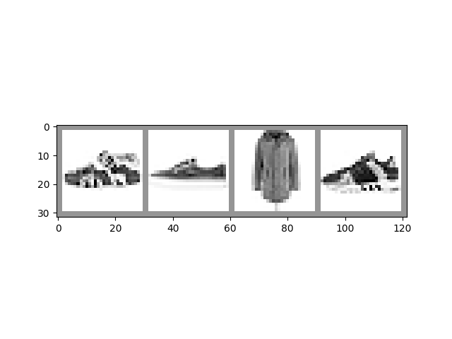
Sandal  Sneaker  Coat  Sneaker

The Model

The model we’ll use in this example is a variant of LeNet-5 - it should be familiar if you’ve watched the previous videos in this series.

import torch.nn as nn
import torch.nn.functional as F

# PyTorch models inherit from torch.nn.Module
class GarmentClassifier(nn.Module):
    def __init__(self):
        super(GarmentClassifier, self).__init__()
        self.conv1 = nn.Conv2d(1, 6, 5)
        self.pool = nn.MaxPool2d(2, 2)
        self.conv2 = nn.Conv2d(6, 16, 5)
        self.fc1 = nn.Linear(16 * 4 * 4, 120)
        self.fc2 = nn.Linear(120, 84)
        self.fc3 = nn.Linear(84, 10)

    def forward(self, x):
        x = self.pool(F.relu(self.conv1(x)))
        x = self.pool(F.relu(self.conv2(x)))
        x = x.view(-1, 16 * 4 * 4)
        x = F.relu(self.fc1(x))
        x = F.relu(self.fc2(x))
        x = self.fc3(x)
        return x


model = GarmentClassifier()

Loss Function

For this example, we’ll be using a cross-entropy loss. For demonstration purposes, we’ll create batches of dummy output and label values, run them through the loss function, and examine the result.

loss_fn = torch.nn.CrossEntropyLoss()

# NB: Loss functions expect data in batches, so we're creating batches of 4
# Represents the model's confidence in each of the 10 classes for a given input
dummy_outputs = torch.rand(4, 10)
# Represents the correct class among the 10 being tested
dummy_labels = torch.tensor([1, 5, 3, 7])

print(dummy_outputs)
print(dummy_labels)

loss = loss_fn(dummy_outputs, dummy_labels)
print('Total loss for this batch: {}'.format(loss.item()))

tensor([[0.7026, 0.1489, 0.0065, 0.6841, 0.4166, 0.3980, 0.9849, 0.6701, 0.4601,
         0.8599],
        [0.7461, 0.3920, 0.9978, 0.0354, 0.9843, 0.0312, 0.5989, 0.2888, 0.8170,
         0.4150],
        [0.8408, 0.5368, 0.0059, 0.8931, 0.3942, 0.7349, 0.5500, 0.0074, 0.0554,
         0.1537],
        [0.7282, 0.8755, 0.3649, 0.4566, 0.8796, 0.2390, 0.9865, 0.7549, 0.9105,
         0.5427]])
tensor([1, 5, 3, 7])
Total loss for this batch: 2.428950071334839

Optimizer

For this example, we’ll be using simple stochastic gradient descent with momentum.

It can be instructive to try some variations on this optimization scheme:

• Learning rate determines the size of the steps the optimizer takes. What does a different learning rate do to the your training results, in terms of accuracy and convergence time?

• Momentum nudges the optimizer in the direction of strongest gradient over multiple steps. What does changing this value do to your results?

• Try some different optimization algorithms, such as averaged SGD, Adagrad, or Adam. How do your results differ?

# Optimizers specified in the torch.optim package
optimizer = torch.optim.SGD(model.parameters(), lr=0.001, momentum=0.9)

The Training Loop

Below, we have a function that performs one training epoch. It enumerates data from the DataLoader, and on each pass of the loop does the following:

• Gets a batch of training data from the DataLoader

• Zeros the optimizer’s gradients

• Performs an inference - that is, gets predictions from the model for an input batch

• Calculates the loss for that set of predictions vs. the labels on the dataset

• Calculates the backward gradients over the learning weights

• Tells the optimizer to perform one learning step - that is, adjust the model’s learning weights based on the observed gradients for this batch, according to the optimization algorithm we chose

• It reports on the loss for every 1000 batches.

• Finally, it reports the average per-batch loss for the last 1000 batches, for comparison with a validation run

def train_one_epoch(epoch_index, tb_writer):
    running_loss = 0.
    last_loss = 0.

    # Here, we use enumerate(training_loader) instead of
    # iter(training_loader) so that we can track the batch
    # index and do some intra-epoch reporting
    for i, data in enumerate(training_loader):
        # Every data instance is an input + label pair
        inputs, labels = data

        # Zero your gradients for every batch!
        optimizer.zero_grad()

        # Make predictions for this batch
        outputs = model(inputs)

        # Compute the loss and its gradients
        loss = loss_fn(outputs, labels)
        loss.backward()

        # Adjust learning weights
        optimizer.step()

        # Gather data and report
        running_loss += loss.item()
        if i % 1000 == 999:
            last_loss = running_loss / 1000 # loss per batch
            print('  batch {} loss: {}'.format(i + 1, last_loss))
            tb_x = epoch_index * len(training_loader) + i + 1
            tb_writer.add_scalar('Loss/train', last_loss, tb_x)
            running_loss = 0.

    return last_loss

Per-Epoch Activity

There are a couple of things we’ll want to do once per epoch:

• Perform validation by checking our relative loss on a set of data that was not used for training, and report this

• Save a copy of the model

Here, we’ll do our reporting in TensorBoard. This will require going to the command line to start TensorBoard, and opening it in another browser tab.

# Initializing in a separate cell so we can easily add more epochs to the same run
timestamp = datetime.now().strftime('%Y%m%d_%H%M%S')
writer = SummaryWriter('runs/fashion_trainer_{}'.format(timestamp))
epoch_number = 0

EPOCHS = 5

best_vloss = 1_000_000.

for epoch in range(EPOCHS):
    print('EPOCH {}:'.format(epoch_number + 1))

    # Make sure gradient tracking is on, and do a pass over the data
    model.train(True)
    avg_loss = train_one_epoch(epoch_number, writer)


    running_vloss = 0.0
    # Set the model to evaluation mode, disabling dropout and using population
    # statistics for batch normalization.
    model.eval()

    # Disable gradient computation and reduce memory consumption.
    with torch.no_grad():
        for i, vdata in enumerate(validation_loader):
            vinputs, vlabels = vdata
            voutputs = model(vinputs)
            vloss = loss_fn(voutputs, vlabels)
            running_vloss += vloss

    avg_vloss = running_vloss / (i + 1)
    print('LOSS train {} valid {}'.format(avg_loss, avg_vloss))

    # Log the running loss averaged per batch
    # for both training and validation
    writer.add_scalars('Training vs. Validation Loss',
                    { 'Training' : avg_loss, 'Validation' : avg_vloss },
                    epoch_number + 1)
    writer.flush()

    # Track best performance, and save the model's state
    if avg_vloss < best_vloss:
        best_vloss = avg_vloss
        model_path = 'model_{}_{}'.format(timestamp, epoch_number)
        torch.save(model.state_dict(), model_path)

    epoch_number += 1

EPOCH 1:
  batch 1000 loss: 1.6334228584356607
  batch 2000 loss: 0.8325267538074403
  batch 3000 loss: 0.7359380583595484
  batch 4000 loss: 0.6198329215242994
  batch 5000 loss: 0.6000315657821484
  batch 6000 loss: 0.555109024874866
  batch 7000 loss: 0.5260250487388112
  batch 8000 loss: 0.4973462742221891
  batch 9000 loss: 0.4781935699362075
  batch 10000 loss: 0.47880298678041433
  batch 11000 loss: 0.45598648857555235
  batch 12000 loss: 0.4327470133750467
  batch 13000 loss: 0.41800182418141046
  batch 14000 loss: 0.4115047634313814
  batch 15000 loss: 0.4211296908891527
LOSS train 0.4211296908891527 valid 0.414460688829422
EPOCH 2:
  batch 1000 loss: 0.3879808729066281
  batch 2000 loss: 0.35912817339546743
  batch 3000 loss: 0.38074520684120944
  batch 4000 loss: 0.3614532373107213
  batch 5000 loss: 0.36850082185724753
  batch 6000 loss: 0.3703581801643886
  batch 7000 loss: 0.38547042514081115
  batch 8000 loss: 0.37846584360170527
  batch 9000 loss: 0.3341486988377292
  batch 10000 loss: 0.3433013284947956
  batch 11000 loss: 0.35607743899174965
  batch 12000 loss: 0.3499939931873523
  batch 13000 loss: 0.33874178926000603
  batch 14000 loss: 0.35130289171106416
  batch 15000 loss: 0.3394507191307202
LOSS train 0.3394507191307202 valid 0.3581162691116333
EPOCH 3:
  batch 1000 loss: 0.3319729989422485
  batch 2000 loss: 0.29558994361863006
  batch 3000 loss: 0.3107374766407593
  batch 4000 loss: 0.3298987646112146
  batch 5000 loss: 0.30858693152241906
  batch 6000 loss: 0.33916381367447684
  batch 7000 loss: 0.3105102765217889
  batch 8000 loss: 0.3011080777524912
  batch 9000 loss: 0.3142058177240979
  batch 10000 loss: 0.31458891937109
  batch 11000 loss: 0.31527258940579483
  batch 12000 loss: 0.31501667268342864
  batch 13000 loss: 0.3011875962628328
  batch 14000 loss: 0.30012811454350596
  batch 15000 loss: 0.31833117976446373
LOSS train 0.31833117976446373 valid 0.3307691514492035
EPOCH 4:
  batch 1000 loss: 0.2786161053752294
  batch 2000 loss: 0.27965198021690596
  batch 3000 loss: 0.28595415444140965
  batch 4000 loss: 0.292985666413857
  batch 5000 loss: 0.3069892351147719
  batch 6000 loss: 0.29902250939945224
  batch 7000 loss: 0.2863366014406201
  batch 8000 loss: 0.2655441066541243
  batch 9000 loss: 0.3045048695363293
  batch 10000 loss: 0.27626545656517554
  batch 11000 loss: 0.2808379335970967
  batch 12000 loss: 0.29241049340573955
  batch 13000 loss: 0.28030834131941446
  batch 14000 loss: 0.2983542350126445
  batch 15000 loss: 0.3009556676162611
LOSS train 0.3009556676162611 valid 0.41686952114105225
EPOCH 5:
  batch 1000 loss: 0.2614263167564495
  batch 2000 loss: 0.2587047562422049
  batch 3000 loss: 0.2642477260621345
  batch 4000 loss: 0.2825975873669813
  batch 5000 loss: 0.26987933717705165
  batch 6000 loss: 0.2759250026817317
  batch 7000 loss: 0.26055969463163275
  batch 8000 loss: 0.29164007206353565
  batch 9000 loss: 0.2893096504513578
  batch 10000 loss: 0.2486029507305684
  batch 11000 loss: 0.2732803234480907
  batch 12000 loss: 0.27927226484491985
  batch 13000 loss: 0.2686819267635074
  batch 14000 loss: 0.24746483912148323
  batch 15000 loss: 0.27903492261294194
LOSS train 0.27903492261294194 valid 0.31206756830215454

To load a saved version of the model:

saved_model = GarmentClassifier()
saved_model.load_state_dict(torch.load(PATH))

Once you’ve loaded the model, it’s ready for whatever you need it for - more training, inference, or analysis.

Note that if your model has constructor parameters that affect model structure, you’ll need to provide them and configure the model identically to the state in which it was saved.

Other Resources

• Docs on the data utilities, including Dataset and DataLoader, at pytorch.org

• A note on the use of pinned memory for GPU training

• Documentation on the datasets available in TorchVision, TorchText, and TorchAudio

• Documentation on the loss functions available in PyTorch

• Documentation on the torch.optim package, which includes optimizers and related tools, such as learning rate scheduling

• A detailed tutorial on saving and loading models

• The Tutorials section of pytorch.org contains tutorials on a broad variety of training tasks, including classification in different domains, generative adversarial networks, reinforcement learning, and more