NLP From Scratch: Classifying Names with a Character-Level RNN

Created On: Mar 24, 2017 | Last Updated: Dec 11, 2024 | Last Verified: Nov 05, 2024

Author: Sean Robertson

This tutorials is part of a three-part series:

• NLP From Scratch: Classifying Names with a Character-Level RNN

• NLP From Scratch: Generating Names with a Character-Level RNN

• NLP From Scratch: Translation with a Sequence to Sequence Network and Attention

We will be building and training a basic character-level Recurrent Neural Network (RNN) to classify words. This tutorial, along with two other Natural Language Processing (NLP) “from scratch” tutorials NLP From Scratch: Generating Names with a Character-Level RNN and NLP From Scratch: Translation with a Sequence to Sequence Network and Attention, show how to preprocess data to model NLP. In particular, these tutorials show how preprocessing to model NLP works at a low level.

A character-level RNN reads words as a series of characters - outputting a prediction and “hidden state” at each step, feeding its previous hidden state into each next step. We take the final prediction to be the output, i.e. which class the word belongs to.

Specifically, we’ll train on a few thousand surnames from 18 languages of origin, and predict which language a name is from based on the spelling.

Recommended Preparation

Before starting this tutorial it is recommended that you have installed PyTorch, and have a basic understanding of Python programming language and Tensors:

• https://pytorch.org/ For installation instructions

• Deep Learning with PyTorch: A 60 Minute Blitz to get started with PyTorch in general and learn the basics of Tensors

• Learning PyTorch with Examples for a wide and deep overview

• PyTorch for Former Torch Users if you are former Lua Torch user

It would also be useful to know about RNNs and how they work:

• The Unreasonable Effectiveness of Recurrent Neural Networks shows a bunch of real life examples

• Understanding LSTM Networks is about LSTMs specifically but also informative about RNNs in general

Preparing Torch

Set up torch to default to the right device use GPU acceleration depending on your hardware (CPU or CUDA).

import torch

# Check if CUDA is available
device = torch.device('cpu')
if torch.cuda.is_available():
    device = torch.device('cuda')

torch.set_default_device(device)
print(f"Using device = {torch.get_default_device()}")

Using device = cuda:0

Preparing the Data

Download the data from here and extract it to the current directory.

Included in the data/names directory are 18 text files named as [Language].txt. Each file contains a bunch of names, one name per line, mostly romanized (but we still need to convert from Unicode to ASCII).

The first step is to define and clean our data. Initially, we need to convert Unicode to plain ASCII to limit the RNN input layers. This is accomplished by converting Unicode strings to ASCII and allowing only a small set of allowed characters.

import string
import unicodedata

allowed_characters = string.ascii_letters + " .,;'"
n_letters = len(allowed_characters)

# Turn a Unicode string to plain ASCII, thanks to https://stackoverflow.com/a/518232/2809427
def unicodeToAscii(s):
    return ''.join(
        c for c in unicodedata.normalize('NFD', s)
        if unicodedata.category(c) != 'Mn'
        and c in allowed_characters
    )

Here’s an example of converting a unicode alphabet name to plain ASCII. This simplifies the input layer

print (f"converting 'Ślusàrski' to {unicodeToAscii('Ślusàrski')}")

converting 'Ślusàrski' to Slusarski

Turning Names into Tensors

Now that we have all the names organized, we need to turn them into Tensors to make any use of them.

To represent a single letter, we use a “one-hot vector” of size <1 x n_letters>. A one-hot vector is filled with 0s except for a 1 at index of the current letter, e.g. "b" = <0 1 0 0 0 ...>.

To make a word we join a bunch of those into a 2D matrix <line_length x 1 x n_letters>.

That extra 1 dimension is because PyTorch assumes everything is in batches - we’re just using a batch size of 1 here.

# Find letter index from all_letters, e.g. "a" = 0
def letterToIndex(letter):
    return allowed_characters.find(letter)

# Turn a line into a <line_length x 1 x n_letters>,
# or an array of one-hot letter vectors
def lineToTensor(line):
    tensor = torch.zeros(len(line), 1, n_letters)
    for li, letter in enumerate(line):
        tensor[li][0][letterToIndex(letter)] = 1
    return tensor

Here are some examples of how to use lineToTensor() for a single and multiple character string.

print (f"The letter 'a' becomes {lineToTensor('a')}") #notice that the first position in the tensor = 1
print (f"The name 'Ahn' becomes {lineToTensor('Ahn')}") #notice 'A' sets the 27th index to 1

The letter 'a' becomes tensor([[[1., 0., 0., 0., 0., 0., 0., 0., 0., 0., 0., 0., 0., 0., 0., 0., 0.,
          0., 0., 0., 0., 0., 0., 0., 0., 0., 0., 0., 0., 0., 0., 0., 0., 0.,
          0., 0., 0., 0., 0., 0., 0., 0., 0., 0., 0., 0., 0., 0., 0., 0., 0.,
          0., 0., 0., 0., 0., 0.]]], device='cuda:0')
The name 'Ahn' becomes tensor([[[0., 0., 0., 0., 0., 0., 0., 0., 0., 0., 0., 0., 0., 0., 0., 0., 0.,
          0., 0., 0., 0., 0., 0., 0., 0., 0., 1., 0., 0., 0., 0., 0., 0., 0.,
          0., 0., 0., 0., 0., 0., 0., 0., 0., 0., 0., 0., 0., 0., 0., 0., 0.,
          0., 0., 0., 0., 0., 0.]],

        [[0., 0., 0., 0., 0., 0., 0., 1., 0., 0., 0., 0., 0., 0., 0., 0., 0.,
          0., 0., 0., 0., 0., 0., 0., 0., 0., 0., 0., 0., 0., 0., 0., 0., 0.,
          0., 0., 0., 0., 0., 0., 0., 0., 0., 0., 0., 0., 0., 0., 0., 0., 0.,
          0., 0., 0., 0., 0., 0.]],

        [[0., 0., 0., 0., 0., 0., 0., 0., 0., 0., 0., 0., 0., 1., 0., 0., 0.,
          0., 0., 0., 0., 0., 0., 0., 0., 0., 0., 0., 0., 0., 0., 0., 0., 0.,
          0., 0., 0., 0., 0., 0., 0., 0., 0., 0., 0., 0., 0., 0., 0., 0., 0.,
          0., 0., 0., 0., 0., 0.]]], device='cuda:0')

Congratulations, you have built the foundational tensor objects for this learning task! You can use a similar approach for other RNN tasks with text.

Next, we need to combine all our examples into a dataset so we can train, test and validate our models. For this, we will use the Dataset and DataLoader classes to hold our dataset. Each Dataset needs to implement three functions: __init__, __len__, and __getitem__.

from io import open
import glob
import os
import time

import torch
from torch.utils.data import Dataset

class NamesDataset(Dataset):

    def __init__(self, data_dir):
        self.data_dir = data_dir #for provenance of the dataset
        self.load_time = time.localtime #for provenance of the dataset
        labels_set = set() #set of all classes

        self.data = []
        self.data_tensors = []
        self.labels = []
        self.labels_tensors = []

        #read all the ``.txt`` files in the specified directory
        text_files = glob.glob(os.path.join(data_dir, '*.txt'))
        for filename in text_files:
            label = os.path.splitext(os.path.basename(filename))[0]
            labels_set.add(label)
            lines = open(filename, encoding='utf-8').read().strip().split('\n')
            for name in lines:
                self.data.append(name)
                self.data_tensors.append(lineToTensor(name))
                self.labels.append(label)

        #Cache the tensor representation of the labels
        self.labels_uniq = list(labels_set)
        for idx in range(len(self.labels)):
            temp_tensor = torch.tensor([self.labels_uniq.index(self.labels[idx])], dtype=torch.long)
            self.labels_tensors.append(temp_tensor)

    def __len__(self):
        return len(self.data)

    def __getitem__(self, idx):
        data_item = self.data[idx]
        data_label = self.labels[idx]
        data_tensor = self.data_tensors[idx]
        label_tensor = self.labels_tensors[idx]

        return label_tensor, data_tensor, data_label, data_item

Here we can load our example data into the NamesDataset

alldata = NamesDataset("data/names")
print(f"loaded {len(alldata)} items of data")
print(f"example = {alldata[0]}")

loaded 20074 items of data
example = (tensor([9], device='cuda:0'), tensor([[[0., 0., 0., 0., 0., 0., 0., 0., 0., 0., 0., 0., 0., 0., 0., 0., 0.,
          0., 0., 0., 0., 0., 0., 0., 0., 0., 0., 0., 0., 0., 0., 0., 0., 0.,
          0., 0., 1., 0., 0., 0., 0., 0., 0., 0., 0., 0., 0., 0., 0., 0., 0.,
          0., 0., 0., 0., 0., 0.]],

        [[0., 0., 0., 0., 0., 0., 0., 1., 0., 0., 0., 0., 0., 0., 0., 0., 0.,
          0., 0., 0., 0., 0., 0., 0., 0., 0., 0., 0., 0., 0., 0., 0., 0., 0.,
          0., 0., 0., 0., 0., 0., 0., 0., 0., 0., 0., 0., 0., 0., 0., 0., 0.,
          0., 0., 0., 0., 0., 0.]],

        [[0., 0., 0., 0., 0., 0., 0., 0., 0., 0., 0., 0., 0., 0., 1., 0., 0.,
          0., 0., 0., 0., 0., 0., 0., 0., 0., 0., 0., 0., 0., 0., 0., 0., 0.,
          0., 0., 0., 0., 0., 0., 0., 0., 0., 0., 0., 0., 0., 0., 0., 0., 0.,
          0., 0., 0., 0., 0., 0.]],

        [[0., 0., 0., 0., 0., 0., 0., 0., 0., 0., 0., 0., 0., 0., 0., 0., 0.,
          0., 0., 0., 1., 0., 0., 0., 0., 0., 0., 0., 0., 0., 0., 0., 0., 0.,
          0., 0., 0., 0., 0., 0., 0., 0., 0., 0., 0., 0., 0., 0., 0., 0., 0.,
          0., 0., 0., 0., 0., 0.]],

        [[0., 0., 0., 0., 0., 0., 0., 0., 0., 0., 0., 0., 0., 0., 0., 0., 0.,
          1., 0., 0., 0., 0., 0., 0., 0., 0., 0., 0., 0., 0., 0., 0., 0., 0.,
          0., 0., 0., 0., 0., 0., 0., 0., 0., 0., 0., 0., 0., 0., 0., 0., 0.,
          0., 0., 0., 0., 0., 0.]],

        [[0., 0., 0., 0., 0., 0., 0., 0., 0., 0., 0., 0., 0., 0., 0., 0., 0.,
          0., 0., 0., 0., 0., 0., 0., 1., 0., 0., 0., 0., 0., 0., 0., 0., 0.,
          0., 0., 0., 0., 0., 0., 0., 0., 0., 0., 0., 0., 0., 0., 0., 0., 0.,
          0., 0., 0., 0., 0., 0.]]], device='cuda:0'), 'Arabic', 'Khoury')

Using the dataset object allows us to easily split the data into train and test sets. Here we create a 80/20

split but the torch.utils.data has more useful utilities. Here we specify a generator since we need to use the

same device as PyTorch defaults to above.

train_set, test_set = torch.utils.data.random_split(alldata, [.85, .15], generator=torch.Generator(device=device).manual_seed(2024))

print(f"train examples = {len(train_set)}, validation examples = {len(test_set)}")

train examples = 17063, validation examples = 3011

Now we have a basic dataset containing 20074 examples where each example is a pairing of label and name. We have also split the dataset into training and testing so we can validate the model that we build.

Creating the Network

Before autograd, creating a recurrent neural network in Torch involved cloning the parameters of a layer over several timesteps. The layers held hidden state and gradients which are now entirely handled by the graph itself. This means you can implement a RNN in a very “pure” way, as regular feed-forward layers.

This CharRNN class implements an RNN with three components. First, we use the nn.RNN implementation. Next, we define a layer that maps the RNN hidden layers to our output. And finally, we apply a softmax function. Using nn.RNN leads to a significant improvement in performance, such as cuDNN-accelerated kernels, versus implementing each layer as a nn.Linear. It also simplifies the implementation in forward().

import torch.nn as nn
import torch.nn.functional as F

class CharRNN(nn.Module):
    def __init__(self, input_size, hidden_size, output_size):
        super(CharRNN, self).__init__()

        self.rnn = nn.RNN(input_size, hidden_size)
        self.h2o = nn.Linear(hidden_size, output_size)
        self.softmax = nn.LogSoftmax(dim=1)

    def forward(self, line_tensor):
        rnn_out, hidden = self.rnn(line_tensor)
        output = self.h2o(hidden[0])
        output = self.softmax(output)

        return output

We can then create an RNN with 57 input nodes, 128 hidden nodes, and 18 outputs:

n_hidden = 128
rnn = CharRNN(n_letters, n_hidden, len(alldata.labels_uniq))
print(rnn)

CharRNN(
  (rnn): RNN(57, 128)
  (h2o): Linear(in_features=128, out_features=18, bias=True)
  (softmax): LogSoftmax(dim=1)
)

After that we can pass our Tensor to the RNN to obtain a predicted output. Subsequently, we use a helper function, label_from_output, to derive a text label for the class.

def label_from_output(output, output_labels):
    top_n, top_i = output.topk(1)
    label_i = top_i[0].item()
    return output_labels[label_i], label_i

input = lineToTensor('Albert')
output = rnn(input) #this is equivalent to ``output = rnn.forward(input)``
print(output)
print(label_from_output(output, alldata.labels_uniq))

tensor([[-2.9390, -2.8275, -2.8058, -3.0319, -2.8306, -2.9352, -2.9732, -2.9896,
         -2.8615, -2.9002, -2.8282, -2.8838, -2.9461, -2.9186, -2.8518, -2.8175,
         -2.8220, -2.9018]], device='cuda:0', grad_fn=<LogSoftmaxBackward0>)
('English', 2)

Training

Training the Network

Now all it takes to train this network is show it a bunch of examples, have it make guesses, and tell it if it’s wrong.

We do this by defining a train() function which trains the model on a given dataset using minibatches. RNNs RNNs are trained similarly to other networks; therefore, for completeness, we include a batched training method here. The loop (for i in batch) computes the losses for each of the items in the batch before adjusting the weights. This operation is repeated until the number of epochs is reached.

import random
import numpy as np

def train(rnn, training_data, n_epoch = 10, n_batch_size = 64, report_every = 50, learning_rate = 0.2, criterion = nn.NLLLoss()):
    """
    Learn on a batch of training_data for a specified number of iterations and reporting thresholds
    """
    # Keep track of losses for plotting
    current_loss = 0
    all_losses = []
    rnn.train()
    optimizer = torch.optim.SGD(rnn.parameters(), lr=learning_rate)

    start = time.time()
    print(f"training on data set with n = {len(training_data)}")

    for iter in range(1, n_epoch + 1):
        rnn.zero_grad() # clear the gradients

        # create some minibatches
        # we cannot use dataloaders because each of our names is a different length
        batches = list(range(len(training_data)))
        random.shuffle(batches)
        batches = np.array_split(batches, len(batches) //n_batch_size )

        for idx, batch in enumerate(batches):
            batch_loss = 0
            for i in batch: #for each example in this batch
                (label_tensor, text_tensor, label, text) = training_data[i]
                output = rnn.forward(text_tensor)
                loss = criterion(output, label_tensor)
                batch_loss += loss

            # optimize parameters
            batch_loss.backward()
            nn.utils.clip_grad_norm_(rnn.parameters(), 3)
            optimizer.step()
            optimizer.zero_grad()

            current_loss += batch_loss.item() / len(batch)

        all_losses.append(current_loss / len(batches) )
        if iter % report_every == 0:
            print(f"{iter} ({iter / n_epoch:.0%}): \t average batch loss = {all_losses[-1]}")
        current_loss = 0

    return all_losses

We can now train a dataset with minibatches for a specified number of epochs. The number of epochs for this example is reduced to speed up the build. You can get better results with different parameters.

start = time.time()
all_losses = train(rnn, train_set, n_epoch=27, learning_rate=0.15, report_every=5)
end = time.time()
print(f"training took {end-start}s")

training on data set with n = 17063
5 (19%):         average batch loss = 0.8816548102676972
10 (37%):        average batch loss = 0.6801934948765246
15 (56%):        average batch loss = 0.5737201840909248
20 (74%):        average batch loss = 0.49455174403065816
25 (93%):        average batch loss = 0.42780510293672097
training took 696.8674302101135s

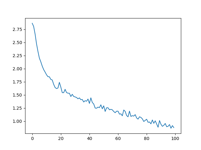
Plotting the Results

Plotting the historical loss from all_losses shows the network learning:

import matplotlib.pyplot as plt
import matplotlib.ticker as ticker

plt.figure()
plt.plot(all_losses)
plt.show()

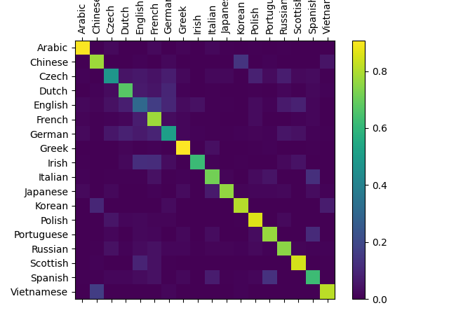
Evaluating the Results

To see how well the network performs on different categories, we will create a confusion matrix, indicating for every actual language (rows) which language the network guesses (columns). To calculate the confusion matrix a bunch of samples are run through the network with evaluate(), which is the same as train() minus the backprop.

def evaluate(rnn, testing_data, classes):
    confusion = torch.zeros(len(classes), len(classes))

    rnn.eval() #set to eval mode
    with torch.no_grad(): # do not record the gradients during eval phase
        for i in range(len(testing_data)):
            (label_tensor, text_tensor, label, text) = testing_data[i]
            output = rnn(text_tensor)
            guess, guess_i = label_from_output(output, classes)
            label_i = classes.index(label)
            confusion[label_i][guess_i] += 1

    # Normalize by dividing every row by its sum
    for i in range(len(classes)):
        denom = confusion[i].sum()
        if denom > 0:
            confusion[i] = confusion[i] / denom

    # Set up plot
    fig = plt.figure()
    ax = fig.add_subplot(111)
    cax = ax.matshow(confusion.cpu().numpy()) #numpy uses cpu here so we need to use a cpu version
    fig.colorbar(cax)

    # Set up axes
    ax.set_xticks(np.arange(len(classes)), labels=classes, rotation=90)
    ax.set_yticks(np.arange(len(classes)), labels=classes)

    # Force label at every tick
    ax.xaxis.set_major_locator(ticker.MultipleLocator(1))
    ax.yaxis.set_major_locator(ticker.MultipleLocator(1))

    # sphinx_gallery_thumbnail_number = 2
    plt.show()



evaluate(rnn, test_set, classes=alldata.labels_uniq)

You can pick out bright spots off the main axis that show which languages it guesses incorrectly, e.g. Chinese for Korean, and Spanish for Italian. It seems to do very well with Greek, and very poorly with English (perhaps because of overlap with other languages).

Exercises

• Get better results with a bigger and/or better shaped network

  • Adjust the hyperparameters to enhance performance, such as changing the number of epochs, batch size, and learning rate

  • Try the nn.LSTM and nn.GRU layers

  • Modify the size of the layers, such as increasing or decreasing the number of hidden nodes or adding additional linear layers

  • Combine multiple of these RNNs as a higher level network

• Try with a different dataset of line -> label, for example:

  • Any word -> language

  • First name -> gender

  • Character name -> writer

  • Page title -> blog or subreddit