In the previous article, we’ve discussed how the SSD algorithm works, covered its implementation details and presented its training process. If you have not read the previous blog post, I encourage you to check it out before continuing.
In this part 2 of the series, we will focus on the mobile-friendly variant of SSD called SSDlite. Our plan is to first go through the main components of the algorithm highlighting the parts that differ from the original SSD, then discuss how the released model was trained and finally provide detailed benchmarks for all the new Object Detection models that we explored.
The SSDlite Network Architecture
The SSDlite is an adaptation of SSD which was first briefly introduced on the MobileNetV2 paper and later reused on the MobileNetV3 paper. Because the main focus of the two papers was to introduce novel CNN architectures, most of the implementation details of SSDlite were not clarified. Our code follows all the details presented on the two papers and where necessary fills the gaps from the official implementation.
As noted before, the SSD is a family of models because one can configure it with different backbones (such as VGG, MobileNetV3 etc) and different Heads (such as using regular convolutions, separable convolutions etc). Thus many of the SSD components remain the same in SSDlite. Below we discuss only those that are different
Classification and Regression Heads
Following the Section 6.2 of the MobileNetV2 paper, SSDlite replaces the regular convolutions used on the original Heads with separable convolutions. Consequently, our implementation introduces new heads that use 3×3 Depthwise convolutions and 1×1 projections. Since all other components of the SSD method remain the same, to create an SSDlite model our implementation initializes the SSDlite head and passes it directly to the SSD constructor.
Backbone Feature Extractor
Our implementation introduces a new class for building MobileNet feature extractors. Following the Section 6.3 of the MobileNetV3 paper, the backbone returns the output of the expansion layer of the Inverted Bottleneck block which has an output stride of 16 and the output of the layer just before the pooling which has an output stride of 32. Moreover, all extra blocks of the backbone are replaced with lightweight equivalents which use a 1×1 compression, a separable 3×3 convolution with stride 2 and a 1×1 expansion. Finally to ensure that the heads have enough prediction power even when small width multipliers are used, the minimum depth size of all convolutions is controlled by the min_depth hyperparameter.
The SSDlite320 MobileNetV3-Large model

This section discusses the configuration of the provided SSDlite pre-trained model along with the training processes followed to replicate the paper results as closely as possible.
Training process
All of the hyperparameters and scripts used to train the model on the COCO dataset can be found in our references folder. Here we discuss the most notable details of the training process.
Tuned Hyperparameters
Though the papers don’t provide any information on the hyperparameters used for training the models (such as regularization, learning rate and the batch size), the parameters listed in the configuration files on the official repo were good starting points and using cross validation we adjusted them to their optimal values. All the above gave us a significant boost over the baseline SSD configuration.
Data Augmentation
Key important difference of SSDlite comparing to SSD is that the backbone of the first has only a fraction of the weights of the latter. This is why in SSDlite, the Data Augmentation focuses more on making the model robust to objects of variable sizes than trying to avoid overfitting. Consequently, SSDlite uses only a subset of the SSD transformations and this way it avoids the over-regularization of the model.
LR Scheme
Due to the reliance on Data Augmentation to make the model robust to small and medium sized objects, we found that it is particularly beneficial for the training recipe to use large number of epochs. More specifically by using roughly 3x more epochs than SSD we are able to increase our precision by 4.2mAP points and by using a 6x multiplier we improve by 4.9mAP. Increasing further the epochs seems to yield diminishing returns and makes the training too slow and impractical, nevertheless based on the model configuration it seems that the authors of the paper used an equivalent 16x multiplier.
Weight Initialization & Input Scaling & ReLU6
A set of final optimizations that brought our implementation very close to the official one and helped us bridge the accuracy gap was training the backbone from scratch instead of initializing from ImageNet, adapting our weight initialization scheme, changing our Input Scaling and replacing all standard ReLUs added on the SSDlite heads with ReLU6. Note that since we trained the model from random weights, we additionally applied the speed optimization described on the paper of using a reduced tail on the backbone.
Implementation Differences
Comparing the above implementation with the one on the official repo, we’ve identified a few differences. Most of them are minor and they are related to how we initialize the weights (for example Normal initialization vs Truncated Normal), how we parameterize the LR Scheduling (for example smaller vs larger warmup rate, shorter vs longer training) etc. The biggest known difference lies in the way we compute the Classification loss. More specifically the implementation of SSDlite with MobileNetV3 backbone on the official repo doesn’t use the SSD’s Multibox loss but instead uses RetinaNet’s focal loss. This is a rather significant deviation from the paper and since TorchVision already offers a full implementation of RetinaNet, we decided to implement SSDlite using the normal Multi-box SSD loss.
Break down of key accuracy improvements
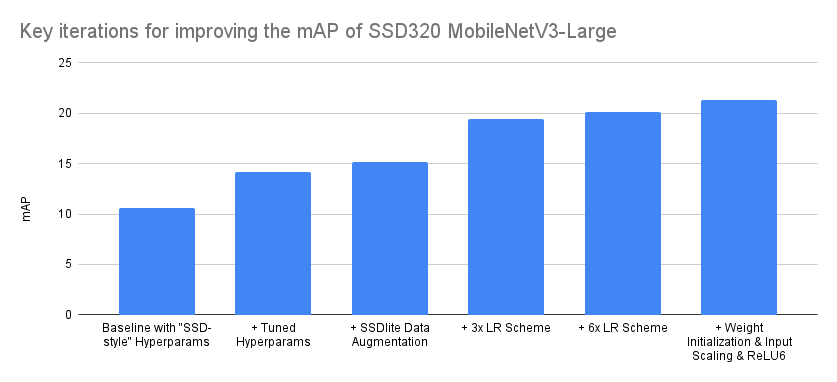
As discussed in previous articles, reproducing research papers and porting them to code is not a journey of monotonically increasing accuracies, especially in cases where the full training and implementation details are not known. Typically the process involves lots of backtracking as one needs to identify those implementation details and parameters that have significant impact on the accuracy from those that don’t. Below we try to visualize the most important iterations that improved our accuracy from the baseline:

| Iteration | mAP |
|---|---|
| Baseline with “SSD-style” Hyperparams | 10.6 |
| + Tuned Hyperparams | 14.2 |
| + SSDlite Data Augmentation | 15.2 |
| + 3x LR Scheme | 19.4 |
| + 6x LR Scheme | 20.1 |
| + Weight Initialization & Input Scaling & ReLU6 | 21.3 |
The order of optimizations presented above is accurate, though a bit idealized in some cases. For example, though different schedulers were tested during the Hyperparameter tuning phase, none of them provided significant improvements and thus we maintained the MultiStepLR which was used in the baseline. Nevertheless while later experimenting with different LR Schemes, we found it beneficial to switch to CosineAnnealingLR, as it required less configuration. Consequently, we believe that the main takeaway from the above summary should be that even by starting with a correct implementation and a set of optimal hyperparams from a model of the same family, there is always accuracy points to be found by optimizing the training recipe and tuning the implementation. Admittedly the above is a rather extreme case where the accuracy doubled, but still in many cases there is a large number of optimizations that can help us push the accuracy significantly.
Benchmarks
Here is how to initialize the two pre-trained models:
ssdlite = torchvision.models.detection.ssdlite320_mobilenet_v3_large(pretrained=True)
ssd = torchvision.models.detection.ssd300_vgg16(pretrained=True)
Below are the benchmarks between the new and selected previous detection models:
| Model | mAP | Inference on CPU (sec) | # Params (M) |
|---|---|---|---|
| SSDlite320 MobileNetV3-Large | 21.3 | 0.0911 | 3.44 |
| SSD300 VGG16 | 25.1 | 0.8303 | 35.64 |
| SSD512 VGG16 (not released) | 28.8 | 2.2494 | 37.08 |
| SSD512 ResNet50 (not released) | 30.2 | 1.1137 | 42.70 |
| Faster R-CNN MobileNetV3-Large 320 FPN (Low-Res) | 22.8 | 0.1679 | 19.39 |
| Faster R-CNN MobileNetV3-Large FPN (High-Res) | 32.8 | 0.8409 | 19.39 |
As we can see, the SSDlite320 MobileNetV3-Large model is by far the fastest and smallest model and thus it’s an excellent candidate for real-world mobile applications. Though its accuracy is lower than the pre-trained low-resolution Faster R-CNN equivalent, the SSDlite framework is adaptable and one can boost its accuracy by introducing heavier heads with more convolutions.
On the other hand, the SSD300 VGG16 model is rather slow and less accurate. This is mainly because of its VGG16 backbone. Though extremely important and influential, the VGG architecture is nowadays quite outdated. Thus though the specific model has historical and research value and hence it’s included in TorchVision, we recommend to users who want high-resolution detectors for real world applications to either combine SSD with alternative backbones (see this example on how to create one) or use one of the Faster R-CNN pre-trained models.
We hope you enjoyed the 2nd and final part of the SSD series. We are looking forward to your feedback.