In TorchVision v0.10, we’ve released two new Object Detection models based on the SSD architecture. Our plan is to cover the key implementation details of the algorithms along with information on how they were trained in a two-part article.
In part 1 of the series, we will focus on the original implementation of the SSD algorithm as described on the Single Shot MultiBox Detector paper. We will briefly give a high-level description of how the algorithm works, then go through its main components, highlight key parts of its code, and finally discuss how we trained the released model. Our goal is to cover all the necessary details to reproduce the model including those optimizations which are not covered on the paper but are part on the original implementation.
How Does SSD Work?
Reading the aforementioned paper is highly recommended but here is a quick oversimplified refresher. Our target is to detect the locations of objects in an image along with their categories. Here is the Figure 5 from the SSD paper with prediction examples of the model:
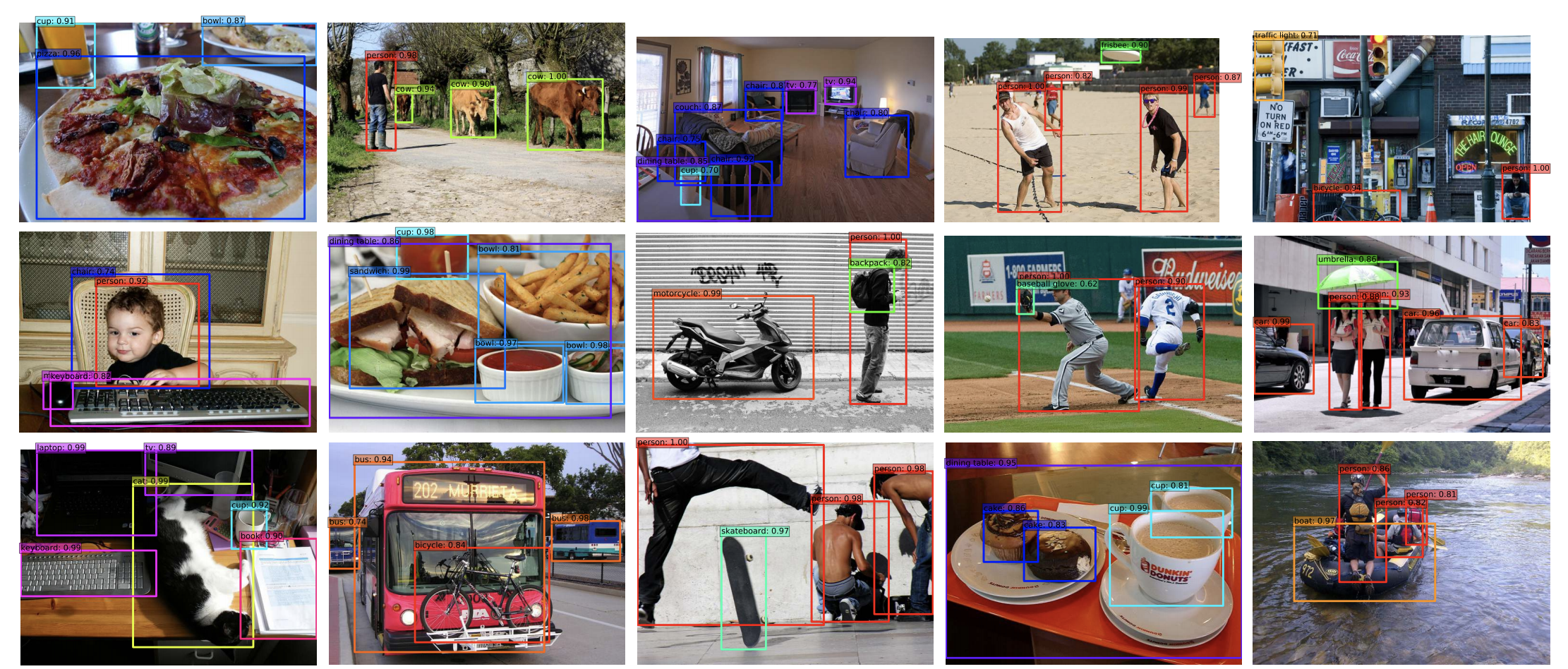
The SSD algorithm uses a CNN backbone, passes the input image through it and takes the convolutional outputs from different levels of the network. The list of these outputs are called feature maps. These feature maps are then passed through the Classification and Regression heads which are responsible for predicting the class and the location of the boxes.
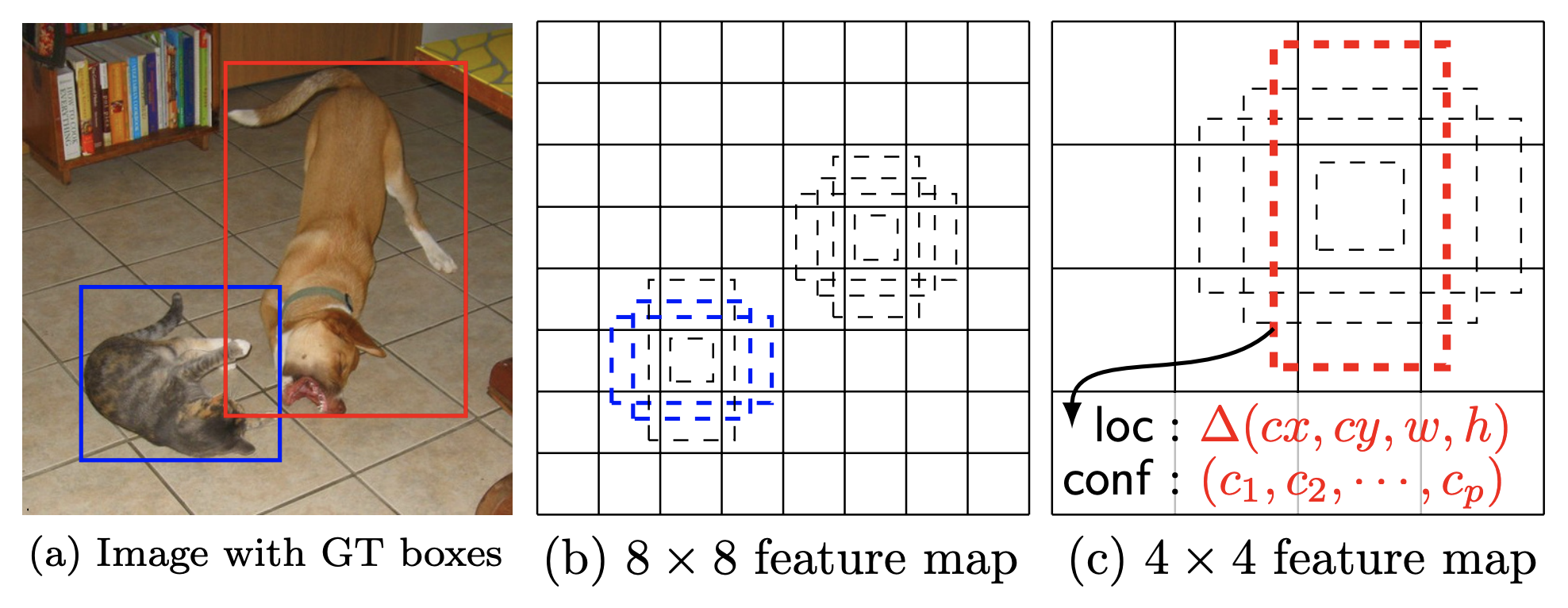
Since the feature maps of each image contain outputs from different levels of the network, their size varies and thus they can capture objects of different dimensions. On top of each, we tile several default boxes which can be thought as our rough prior guesses. For each default box, we predict whether there is an object (along with its class) and its offset (correction over the original location). During training time, we need to first match the ground truth to the default boxes and then we use those matches to estimate our loss. During inference, similar prediction boxes are combined to estimate the final predictions.
The SSD Network Architecture
In this section, we will discuss the key components of SSD. Our code follows closely the paper and makes use of many of the undocumented optimizations included in the official implementation.
DefaultBoxGenerator
The DefaultBoxGenerator class is responsible for generating the default boxes of SSD and operates similarly to the AnchorGenerator of FasterRCNN (for more info on their differences see pages 4-6 of the paper). It produces a set of predefined boxes of specific width and height which are tiled across the image and serve as the first rough prior guesses of where objects might be located. Here is Figure 1 from the SSD paper with a visualization of ground truths and default boxes:
The class is parameterized by a set of hyperparameters that control their shape and tiling. The implementation will provide automatically good guesses with the default parameters for those who want to experiment with new backbones/datasets but one can also pass optimized custom values.
SSDMatcher
The SSDMatcher class extends the standard Matcher used by FasterRCNN and it is responsible for matching the default boxes to the ground truth. After estimating the IoUs of all combinations, we use the matcher to find for each default box the best candidate ground truth with overlap higher than the IoU threshold. The SSD version of the matcher has an extra step to ensure that each ground truth is matched with the default box that has the highest overlap. The results of the matcher are used in the loss estimation during the training process of the model.
Classification and Regression Heads
The SSDHead class is responsible for initializing the Classification and Regression parts of the network. Here are a few notable details about their code:
- Both the Classification and the Regression head inherit from the same class which is responsible for making the predictions for each feature map.
- Each level of the feature map uses a separate 3×3 Convolution to estimate the class logits and box locations.
- The number of predictions that each head makes per level depends on the number of default boxes and the sizes of the feature maps.
Backbone Feature Extractor
The feature extractor reconfigures and enhances a standard VGG backbone with extra layers as depicted on the Figure 2 of the SSD paper:
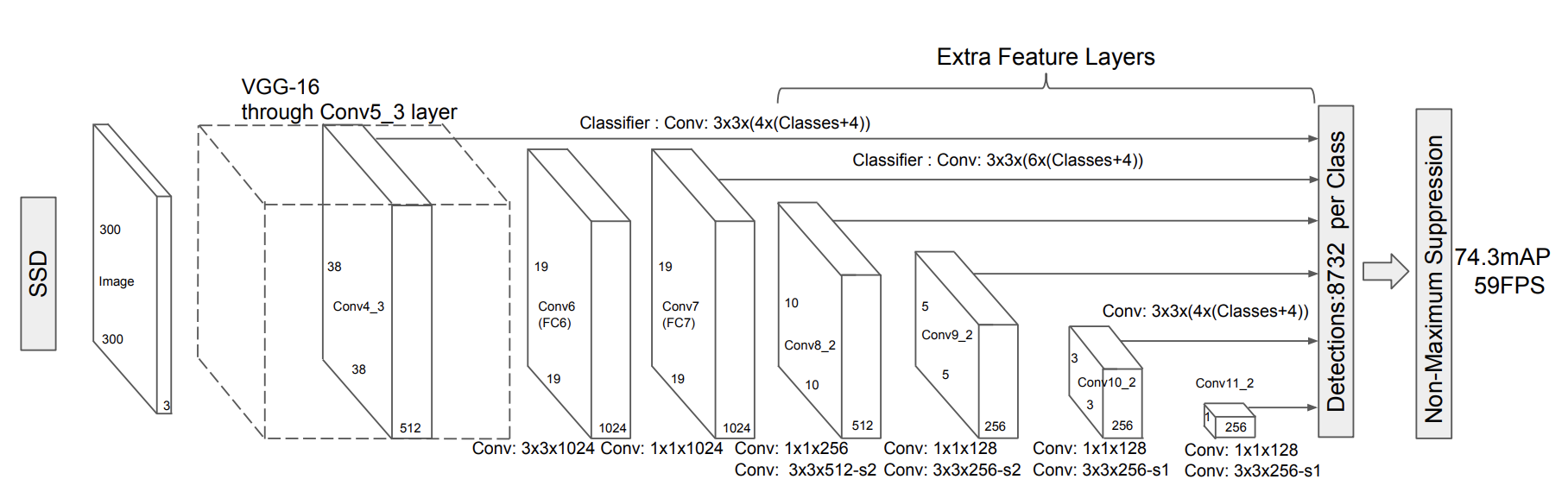
The class supports all VGG models of TorchVision and one can create a similar extractor class for other types of CNNs (see this example for ResNet). Here are a few implementation details of the class:
- Patching the
ceil_mode parameterof the 3rd Maxpool layer is necessary to get the same feature map sizes as the paper. This is due to small differences between PyTorch and the original Caffe implementation of the model. - It adds a series of extra feature layerson top of VGG. If the highres parameter is
Trueduring its construction, it will append an extra convolution. This is useful for the SSD512 version of the model. - As discussed on section 3 of the paper, the fully connected layers of the original VGG are converted to convolutions with the first one using Atrous. Moreover maxpool5’s stride and kernel size is modified.
- As described on section 3.1, L2 normalization is used on the output of conv4_3 and a set of learnable weights are introduced to control its scaling.
SSD Algorithm
The final key piece of the implementation is on the SSD class. Here are some notable details:
- The algorithm is parameterized by a set of arguments similar to other detection models. The mandatory parameters are: the backbone which is responsible for estimating the feature maps, the
anchor_generatorwhich should be a configured instance of theDefaultBoxGeneratorclass, the size to which the input images will be resized and thenum_classesfor classification excluding the background. - If a head is not provided, the constructor will initialize the default
SSDHead. To do so, we need to know the number of output channels for each feature map produced by the backbone. Initially we try to retrieve this information from the backbone but if not available we will dynamically estimate it. - The algorithm reuses the standard BoxCoder class used by other Detection models. The class is responsible for encoding and decoding the bounding boxes and is configured to use the same prior variances as the original implementation.
- Though we reuse the standard GeneralizedRCNNTransform class to resize and normalize the input images, the SSD algorithm configures it to ensure that the image size will remain fixed.
Here are the two core methods of the implementation:
- The
compute_lossmethod estimates the standard Multi-box loss as described on page 5 of the SSD paper. It uses the smooth L1 loss for regression and the standard cross-entropy loss with hard-negative sampling for classification. - As in all detection models, the forward method currently has different behaviour depending on whether the model is on training or eval mode. It starts by resizing & normalizing the input images and then passes them through the backbone to get the feature maps. The feature maps are then passed through the head to get the predictions and then the method generates the default boxes.
- If the model is on training mode, the forward will estimate the IoUs of the default boxes with the ground truth, use the
SSDmatcherto produce matches and finally estimate the losses by calling thecompute_loss method. - If the model is on eval mode, we first select the best detections by keeping only the ones that pass the score threshold, select the most promising boxes and run NMS to clean up and select the best predictions. Finally we postprocess the predictions to resize them to the original image size.
- If the model is on training mode, the forward will estimate the IoUs of the default boxes with the ground truth, use the
The SSD300 VGG16 Model
The SSD is a family of models because it can be configured with different backbones and different Head configurations. In this section, we will focus on the provided SSD pre-trained model. We will discuss the details of its configuration and the training process used to reproduce the reported results.
Training process
The model was trained using the COCO dataset and all of its hyper-parameters and scripts can be found in our references folder. Below we provide details on the most notable aspects of the training process.
Paper Hyperparameters
In order to achieve the best possible results on COCO, we adopted the hyperparameters described on the section 3 of the paper concerning the optimizer configuration, the weight regularization etc. Moreover we found it useful to adopt the optimizations that appear in the official implementation concerning the tiling configuration of the DefaultBox generator. This optimization was not described in the paper but it was crucial for improving the detection precision of smaller objects.
Data Augmentation
Implementing the SSD Data Augmentation strategy as described on page 6 and page 12 of the paper was critical to reproducing the results. More specifically the use of random “Zoom In” and “Zoom Out” transformations make the model robust to various input sizes and improve its precision on the small and medium objects. Finally since the VGG16 has quite a few parameters, the photometric distortions included in the augmentations have a regularization effect and help avoid the overfitting.
Weight Initialization & Input Scaling
Another aspect that we found beneficial was to follow the weight initialization scheme proposed by the paper. To do that, we had to adapt our input scaling method by undoing the 0-1 scaling performed by ToTensor() and use pre-trained ImageNet weights fitted with this scaling (shoutout to Max deGroot for providing them in his repo). All the weights of new convolutions were initialized using Xavier and their biases were set to zero. After initialization, the network was trained end-to-end.
LR Scheme
As reported on the paper, after applying aggressive data augmentations it’s necessary to train the models for longer. Our experiments confirm this and we had to tweak the Learning rate, batch sizes and overall steps to achieve the best results. Our proposed learning scheme is configured to be rather on the safe side, showed signs of plateauing between the steps and thus one is likely to be able to train a similar model by doing only 66% of our epochs.
Breakdown of Key Accuracy Improvements
It is important to note that implementing a model directly from a paper is an iterative process that circles between coding, training, bug fixing and adapting the configuration until we match the accuracies reported on the paper. Quite often it also involves simplifying the training recipe or enhancing it with more recent methodologies. It is definitely not a linear process where incremental accuracy improvements are achieved by improving a single direction at a time but instead involves exploring different hypothesis, making incremental improvements in different aspects and doing a lot of backtracking.
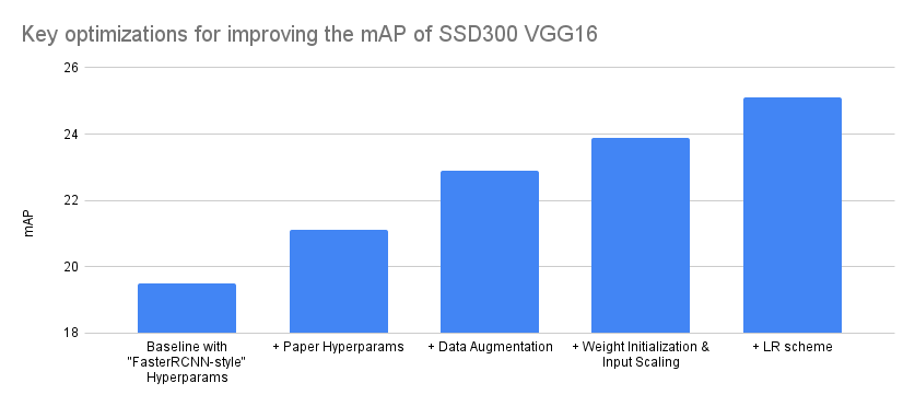
With that in mind, below we try to summarize the optimizations that affected our accuracy the most. We did this by grouping together the various experiments in 4 main groups and attributing the experiment improvements to the closest match. Note that the Y-axis of the graph starts from 18 instead from 0 to make the difference between optimizations more visible:
| Model Configuration | mAP delta | mAP |
|---|---|---|
| Baseline with “FasterRCNN-style” Hyperparams | – | 19.5 |
| + Paper Hyperparams | 1.6 | 21.1 |
| + Data Augmentation | 1.8 | 22.9 |
| + Weight Initialization & Input Scaling | 1 | 23.9 |
| + LR scheme | 1.2 | 25.1 |
Our final model achieves an mAP of 25.1 and reproduces exactly the COCO results reported on the paper. Here is a detailed breakdown of the accuracy metrics.
We hope you found the part 1 of the series interesting. On the part 2, we will focus on the implementation of SSDlite and discuss its differences from SSD. Until then, we are looking forward to your feedback.