Large model training using a cloud native approach is of growing interest for many enterprises given the emergence and success of foundation models. Some AI practitioners may assume that the only way they can achieve high GPU utilization for distributed training jobs is to run them on HPC systems, such as those inter-connected with Infiniband and may not consider Ethernet connected systems. We demonstrate how the latest distributed training technique, Fully Sharded Data Parallel (FSDP) from PyTorch, successfully scales to models of size 10B+ parameters using commodity Ethernet networking in IBM Cloud.
PyTorch FSDP Scaling
As models get larger, the standard techniques for data parallel training work only if the GPU can hold a full replica of the model, along with its training state (optimizer, activations, etc.). However, GPU memory increases have not kept up with the model size increases and new techniques for training such models have emerged (e.g., Fully Sharded Data Parallel, DeepSpeed), which allow us to efficiently distribute the model and data over multiple GPUs during training. In this blog post, we demonstrate a path to achieve remarkable scaling of model training to 64 nodes (512 GPUs) using PyTorch native FSDP APIs as we increase model sizes to 11B.
What is Fully Sharded Data Parallel?
FSDP extends the distributed data parallel training (DDP) approach by sharding model parameters, gradient and optimizer states into K FSDP units, determined by using a wrapping policy. FSDP achieves large model training efficiency in terms of resources and performance by significantly reducing the memory footprint on each GPU and overlapping computation and communication.
Resource efficiency is achieved with memory footprint reduction by having all GPUs own a portion of each FSDP unit. To process a given FSDP unit, all GPUs share their locally owned portion via all_gather communication calls.
Performance efficiency is accomplished by overlapping all_gather communication calls for upcoming FSDP units with computation of the current FSDP unit. Once the current FSDP unit has been processed, the non-locally owned parameters are dropped, freeing memory for the upcoming FSDP units. This process achieves training efficiency by the overlap of computation and communication, while also reducing the peak memory needed by each GPU.
In what follows, we demonstrate how FSDP allows us to keep hundreds of GPUs highly utilized throughout a distributed training job, while running over standard Ethernet networking (system description towards the end of the blog). We chose the T5 architecture for our experiments and leveraged the code from the FSDP workshop. In each of our experiments, we start with a single node experiment to create a baseline and report the metric seconds/iteration normalized by the batch size as well as compute the teraflops based on the Megatron-LM paper (see Appendix for details of teraflop computation for T5). Our experiments aim to maximize the batch size (while avoiding cudaMalloc retries) to take full advantage of overlap in computation and communications, as discussed below. Scaling is defined as the ratio of the seconds/iteration normalized by batch size for N nodes versus a single node, representing how well we can utilize the additional GPUs as more nodes are added.
Experimental Results
Our first set of experiments using the T5-3B configuration (mixed precision with BF16, activation checkpointing, and transformer wrapping policy) demonstrated scaling efficiency of 95% as we increased the number of GPUs from 8 to 512 (1 to 64 nodes, respectively). We achieved these results without any modifications to the existing FSDP APIs. We observed that, for this scale, over Ethernet based network, there is sufficient bandwidth to enable continuous overlap of communication and computation.
However, when we increased the T5 model size to 11B, the scaling efficiency declined substantially to 20%. The PyTorch profiler shows that overlap of communication and computation was very limited. Further investigation into the network bandwidth usage revealed that the poor overlap is being caused by latency in the communication of individual packets and not the bandwidth required (in fact, our peak bandwidth utilization is 1/4th of that available). This led us to hypothesize that if we can increase the compute time by increasing the batch size, we can better overlap communication and computation. However, given we are already at maximum GPU memory allocation, we must identify opportunities to rebalance the memory allocation to allow for increase in batch size. We identified that the model state was being allocated a lot more memory than was needed. The primary function of these reservations is to have pre-reserved memory ready to aggressively send/receive tensors during the communication periods and too few buffers can result in increased wait times, whereas too many buffers result in smaller batch sizes.
To achieve better efficiency, the PyTorch distributed team introduced a new control knob, the rate_limiter which controls how much memory is allocated for send/receive of tensors, alleviating the memory pressure and providing room for higher batch sizes. In our case, the rate_limiter could increase the batch size from 20 to 50, thus increasing compute time by 2.5x and allowing for much greater overlap of communication and computation. With this fix, we increased the scaling efficiency to >75% (at 32 nodes)!
Continued investigation into the factors limiting scaling efficiency uncovered that the rate limiter was creating a recurring pipeline bubble of GPU idle time. This was due to the rate limiter using a block and flush approach for the allocation and release of each set of memory buffers. By waiting for the entire block to complete before initiating a new all_gather, the GPU was idling at the start of each block, while waiting for the new set of all_gather parameters to arrive. This bubble was alleviated by moving to a sliding window approach. Upon the completion of a single all_gather step and its computation (rather than a block of them), the memory is freed and the next all_gather is immediately issued in a much more uniform manner. This improvement eliminated the pipeline bubble and boosted the scaling efficiencies to >90% (at 32 nodes).
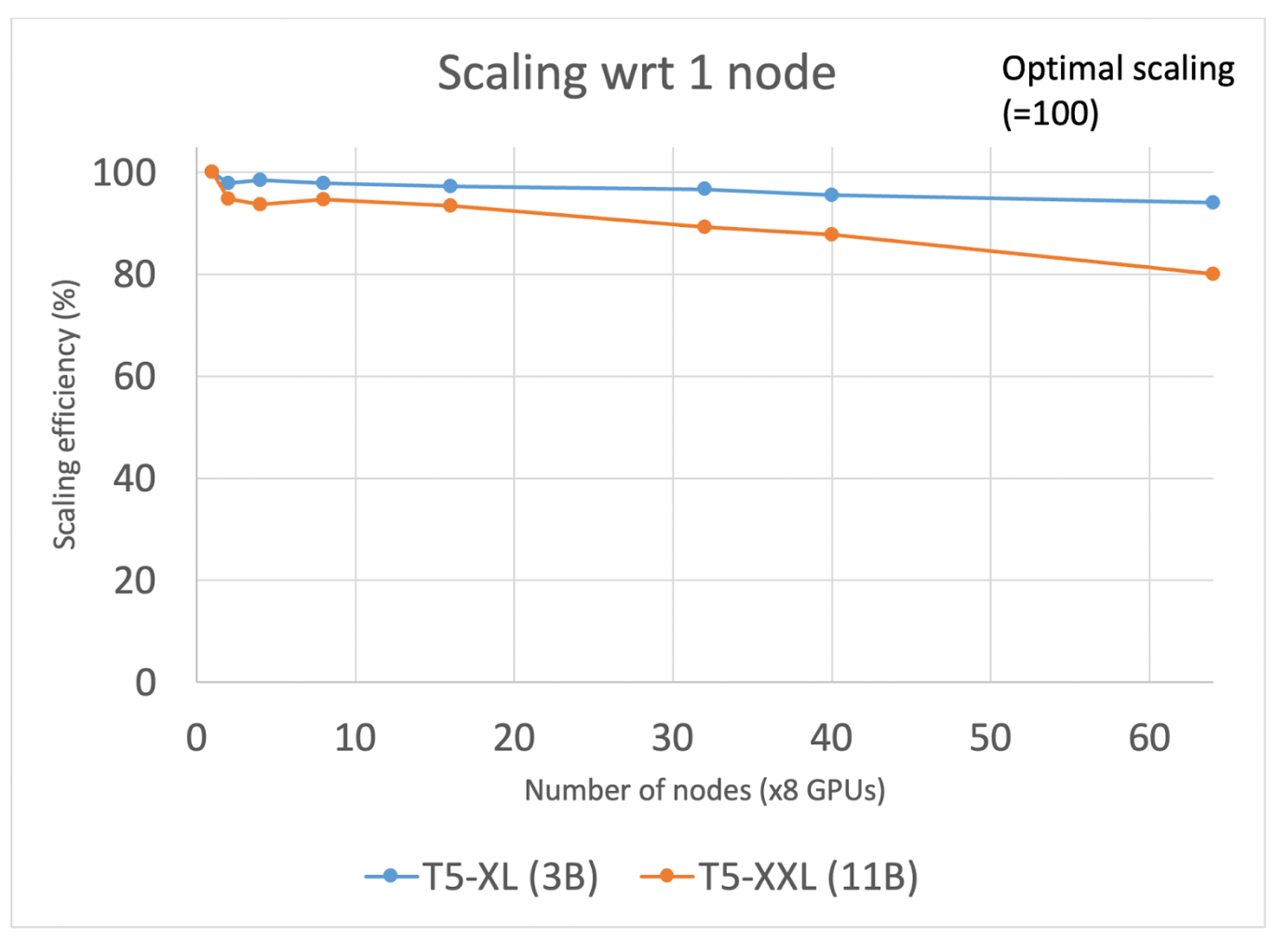
Figure 1: Scaling of T5-XL (3B) and T5-XXL (11B) from 1 node to 64 nodes
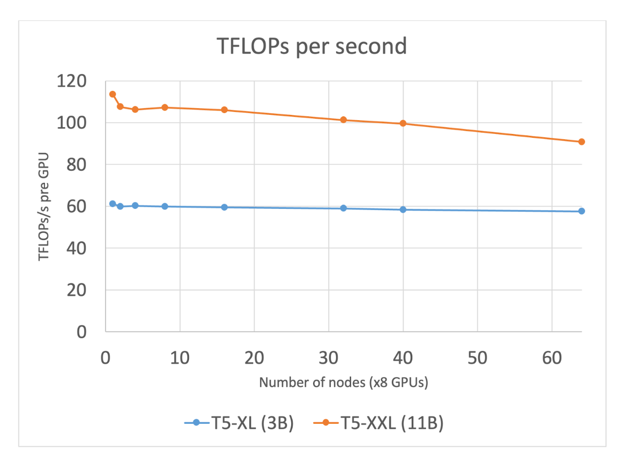
Figure 2: TFLOPs/sec usage for T5-XL(3B) and T5-XXL (11B) as we increase number of nodes
IBM Cloud AI System and Middleware
The AI infrastructure used for this work is a large-scale AI system on IBM Cloud consisting of nearly 200 nodes, each node with 8 NVIDIA A100 80GB cards, 96 vCPUs, and 1.2TB CPU RAM. The GPU cards within a node are connected via NVLink with a card-to-card bandwidth of 600GBps. Nodes are connected by 2 x 100Gbps Ethernet links with SRIOV based TCP/IP stack, providing a usable bandwidth of 120Gbps.
The IBM Cloud AI System has been production-ready since May of 2022 and is configured with the OpenShift container platform to run AI workloads. We also built a software stack for production AI workloads that provide end-to-end tools for training workloads. The middleware leverages Ray for pre and post processing workloads and PyTorch for training of models. We also integrate a Kubernetes native scheduler, MCAD, that manages multiple jobs with job queuing, gang scheduling, prioritization, and quota management. A multi-NIC CNI discovers all available network interfaces and handles them as a single NIC pool enabling optimized use of the network interfaces in Kubernetes. Finally, CodeFlare CLI supports a single pane for observability of the full stack using a desktop CLI (e.g., GPU utilization, application metrics like loss, gradient norm).
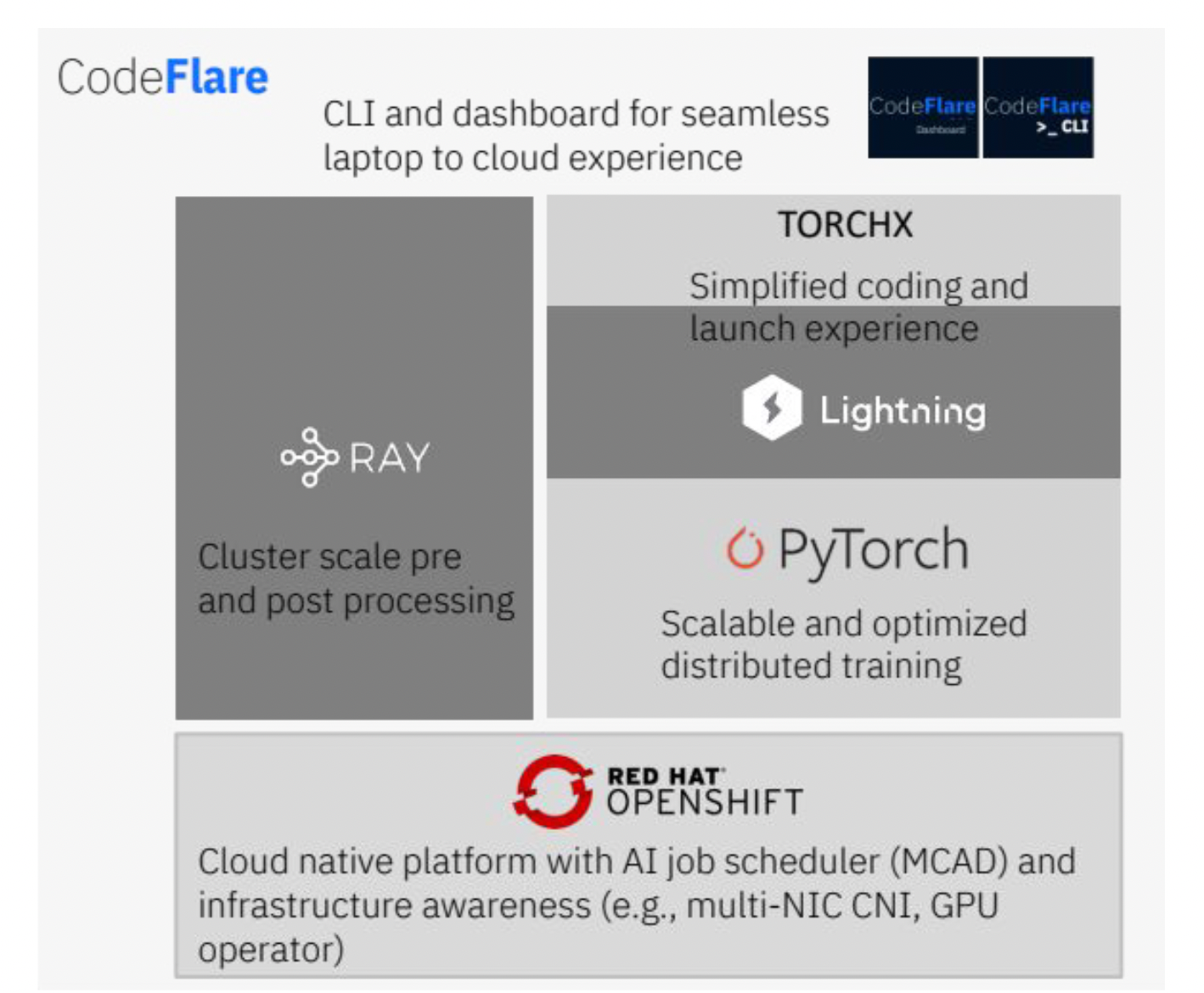
Figure 3: Foundation Model Middleware Stack
Conclusion and Future Work
In conclusion, we demonstrated how we can achieve remarkable scaling of FSDP APIs over non-InfiniBand networks. We identified the bottleneck that had limited scaling to less than 20% efficiency for 11B parameter model training. After identifying the issue, we were able to correct this with a new rate limiter control to ensure a more optimal balance of reserved memory and communication overlap relative to compute time. With this improvement, we were able to achieve 90% scaling efficiency (a 4.5x improvement), at 256 GPUs and 80% at 512 GPUs for training of the 11B parameter model. In addition, the 3B parameter model scales extremely well with 95% efficiency even as we increase the number of GPUs to 512.
This is a first in the industry to achieve such scaling efficiencies for up to 11B parameter models using Kubernetes with vanilla Ethernet and PyTorch native FSDP API’s. This improvement enables users to train huge models on a Hybrid Cloud platform in a cost efficient and sustainable manner.
We plan on continuing to investigate scaling with decoder only models and increasing the size of these models to 100B+ parameters. From a system design perspective, we are exploring capabilities such as RoCE and GDR that can improve latencies of communications over Ethernet networks.
Acknowledgements
This blog was possible because of contributions from both PyTorch Distributed and IBM Research teams.
From the PyTorch Distributed team, we would like to thank Less Wright, Hamid Shojanazeri, Geeta Chauhan, Shen Li, Rohan Varma, Yanli Zhao, Andrew Gu, Anjali Sridhar, Chien-Chin Huang, and Bernard Nguyen.
From the IBM Research team, we would like to thank Linsong Chu, Sophia Wen, Lixiang (Eric) Luo, Marquita Ellis, Davis Wertheimer, Supriyo Chakraborty, Raghu Ganti, Mudhakar Srivatsa, Seetharami Seelam, Carlos Costa, Abhishek Malvankar, Diana Arroyo, Alaa Youssef, Nick Mitchell.
Appendix
Teraflop computation
The T5-XXL (11B) architecture has two types of T5 blocks, one is an encoder and the second is a decoder. Following the approach of Megatron-LM, where each matrix multiplication requires 2m×k×n FLOPs, where the first matrix is of size m×k and the second is k×n. The encoder block consists of self-attention and feed forward layers, whereas the decoder block consists of self-attention, cross-attention, and feed forward layers.
The attention (both self and cross) block consists of a QKV projection, which requires 6Bsh2 operations, an attention matrix computation requiring 2Bs2h operations, an attention over values which needs 2Bs2h computations, and the post-attention linear projection requires 2Bsh2 operations. Finally, the feed forward layer requires 15Bsh2 operations.
The total for an encoder block is 23Bsh2+4Bs2h, whereas for a decoder block, it comes to 31Bsh2+8Bs2h. With a total of 24 encoder and 24 decoder blocks and 2 forward passes (as we discard the activations) and one backward pass (equivalent to two forward passes), the final FLOPs computation comes to be 96×(54Bsh2+ 12Bs2h) + 6BshV. Here, B is the batch size per GPU, s is sequence length, h is hidden state size, and V is vocabulary size. We repeat a similar computation for T5-XL (3B) architecture, which is slightly different.