PyTorch Profiler v1.9 has been released! The goal of this new release (previous PyTorch Profiler release) is to provide you with new state-of-the-art tools to help diagnose and fix machine learning performance issues regardless of whether you are working on one or numerous machines. The objective is to target the execution steps that are the most costly in time and/or memory, and visualize the work load distribution between GPUs and CPUs.
Here is a summary of the five major features being released:
- Distributed Training View: This helps you understand how much time and memory is consumed in your distributed training job. Many issues occur when you take a training model and split the load into worker nodes to be run in parallel as it can be a black box. The overall model goal is to speed up model training. This distributed training view will help you diagnose and debug issues within individual nodes.
- Memory View: This view allows you to understand your memory usage better. This tool will help you avoid the famously pesky Out of Memory error by showing active memory allocations at various points of your program run.
- GPU Utilization Visualization: This tool helps you make sure that your GPU is being fully utilized.
- Cloud Storage Support: Tensorboard plugin can now read profiling data from Azure Blob Storage, Amazon S3, and Google Cloud Platform.
- Jump to Source Code: This feature allows you to visualize stack tracing information and jump directly into the source code. This helps you quickly optimize and iterate on your code based on your profiling results.
Getting Started with PyTorch Profiling Tool
PyTorch includes a profiling functionality called « PyTorch Profiler ». The PyTorch Profiler tutorial can be found here.
To instrument your PyTorch code for profiling, you must:
$ pip install torch-tb-profiler
import torch.profiler as profiler
With profiler.profile(XXXX)
Comments:
• For CUDA and CPU profiling, see below:
with torch.profiler.profile(
activities=[
torch.profiler.ProfilerActivity.CPU,
torch.profiler.ProfilerActivity.CUDA],
• With profiler.record_function(“$NAME”): allows putting a decorator (a tag associated to a name) for a block of function
• Profile_memory=True parameter under profiler.profile allows you to profile CPU and GPU memory footprint
Visualizing PyTorch Model Performance using PyTorch Profiler
Distributed Training
Recent advances in deep learning argue for the value of large datasets and large models, which requires you to scale out model training to more computational resources. Distributed Data Parallel (DDP) and NVIDIA Collective Communications Library (NCCL) are the widely adopted paradigms in PyTorch for accelerating your deep learning training.
In this release of PyTorch Profiler, DDP with NCCL backend is now supported.
Computation/Communication Overview
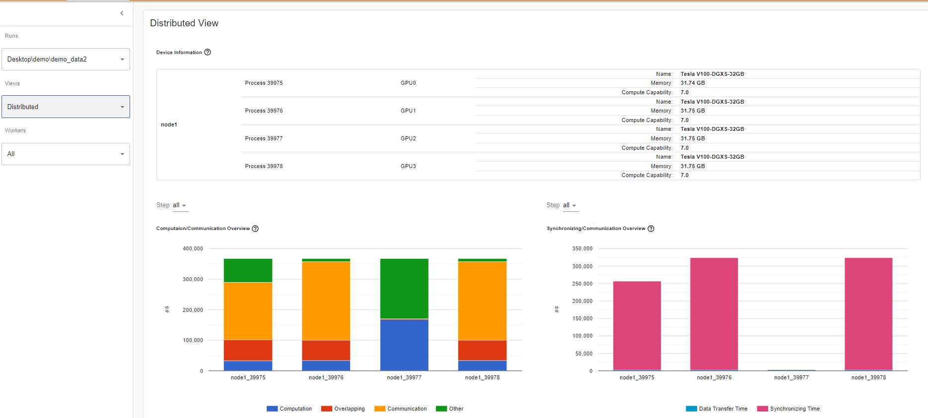
In the Computation/Communication overview under the Distributed training view, you can observe the computation-to-communication ratio of each worker and [load balancer](https://en.wikipedia.org/wiki/Load_balancing_(computing) nodes between worker as measured by granularity.
Scenario 1:
If the computation and overlapping time of one worker is much larger than the others, this may suggest an issue in the workload balance or worker being a straggler. Computation is the sum of kernel time on GPU minus the overlapping time. The overlapping time is the time saved by interleaving communications during computation. The more overlapping time represents better parallelism between computation and communication. Ideally the computation and communication completely overlap with each other. Communication is the total communication time minus the overlapping time. The example image below displays how this scenario appears on Tensorboard.
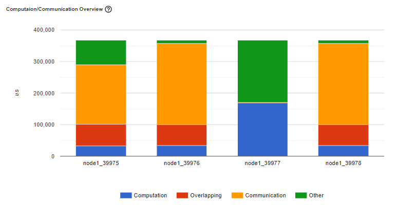
Figure: A straggler example
Scenario 2:
If there is a small batch size (i.e. less computation on each worker) or the data to be transferred is large, the computation-to-communication may also be small and be seen in the profiler with low GPU utilization and long waiting times. This computation/communication view will allow you to diagnose your code to reduce communication by adopting gradient accumulation, or to decrease the communication proportion by increasing batch size. DDP communication time depends on model size. Batch size has no relationship with model size. So increasing batch size could make computation time longer and make computation-to-communication ratio bigger.
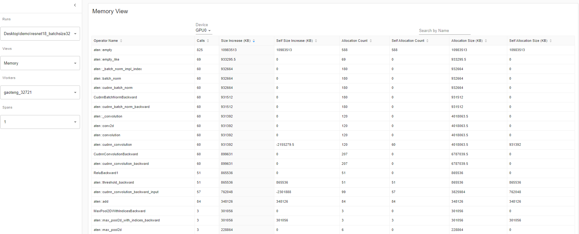
Synchronizing/Communication Overview
In the Synchronizing/Communication view, you can observe the efficiency of communication. This is done by taking the step time minus computation and communication time. Synchronizing time is part of the total communication time for waiting and synchronizing with other workers. The Synchronizing/Communication view includes initialization, data loader, CPU computation, and so on Insights like what is the ratio of total communication is really used for exchanging data and what is the idle time of waiting for data from other workers can be drawn from this view.
For example, if there is an inefficient workload balance or straggler issue, you’ll be able to identify it in this Synchronizing/Communication view. This view will show several workers’ waiting time being longer than others.

This table view above allows you to see the detailed statistics of all communication ops in each node. This allows you to see what operation types are being called, how many times each op is called, what is the size of the data being transferred by each op, etc.
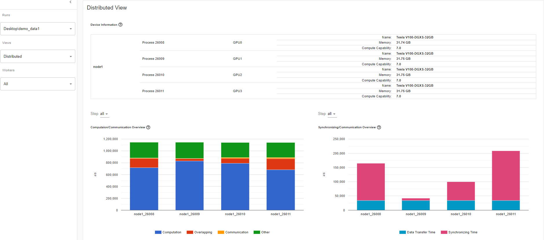
Memory View:
This memory view tool helps you understand the hardware resource consumption of the operators in your model. Understanding the time and memory consumption on the operator-level allows you to resolve performance bottlenecks and in turn, allow your model to execute faster. Given limited GPU memory size, optimizing the memory usage can:
- Allow bigger model which can potentially generalize better on end level tasks.
- Allow bigger batch size. Bigger batch sizes increase the training speed.
The profiler records all the memory allocation during the profiler interval. Selecting the “Device” will allow you to see each operator’s memory usage on the GPU side or host side. You must enable profile_memory=True to generate the below memory data as shown here.
With torch.profiler.profile(
Profiler_memory=True # this will take 1 – 2 minutes to complete.
)
Important Definitions:
• “Size Increase” displays the sum of all allocation bytes and minus all the memory release bytes.
• “Allocation Size” shows the sum of all allocation bytes without considering the memory release.
• “Self” means the allocated memory is not from any child operators, instead by the operator itself.
GPU Metric on Timeline:
This feature will help you debug performance issues when one or more GPU are underutilized. Ideally, your program should have high GPU utilization (aiming for 100% GPU utilization), minimal CPU to GPU communication, and no overhead.
Overview: The overview page highlights the results of three important GPU usage metrics at different levels (i.e. GPU Utilization, Est. SM Efficiency, and Est. Achieved Occupancy). Essentially, each GPU has a bunch of SM each with a bunch of warps that can execute a bunch of threads concurrently. Warps execute a bunch because the amount depends on the GPU. But at a high level, this GPU Metric on Timeline tool allows you can see the whole stack, which is useful.
If the GPU utilization result is low, this suggests a potential bottleneck is present in your model. Common reasons:
•Insufficient parallelism in kernels (i.e., low batch size)
•Small kernels called in a loop. This is to say the launch overheads are not amortized
•CPU or I/O bottlenecks lead to the GPU not receiving enough work to keep busy
Looking of the overview page where the performance recommendation section is where you’ll find potential suggestions on how to increase that GPU utilization. In this example, GPU utilization is low so the performance recommendation was to increase batch size. Increasing batch size 4 to 32, as per the performance recommendation, increased the GPU Utilization by 60.68%.
GPU Utilization: the step interval time in the profiler when a GPU engine was executing a workload. The high the utilization %, the better. The drawback of using GPU utilization solely to diagnose performance bottlenecks is it is too high-level and coarse. It won’t be able to tell you how many Streaming Multiprocessors are in use. Note that while this metric is useful for detecting periods of idleness, a high value does not indicate efficient use of the GPU, only that it is doing anything at all. For instance, a kernel with a single thread running continuously will get a GPU Utilization of 100%
Estimated Stream Multiprocessor Efficiency (Est. SM Efficiency) is a finer grained metric, it indicates what percentage of SMs are in use at any point in the trace This metric reports the percentage of time where there is at least one active warp on a SM and those that are stalled (NVIDIA doc). Est. SM Efficiency also has it’s limitation. For instance, a kernel with only one thread per block can’t fully use each SM. SM Efficiency does not tell us how busy each SM is, only that they are doing anything at all, which can include stalling while waiting on the result of a memory load. To keep an SM busy, it is necessary to have a sufficient number of ready warps that can be run whenever a stall occurs
Estimated Achieved Occupancy (Est. Achieved Occupancy) is a layer deeper than Est. SM Efficiency and GPU Utilization for diagnosing performance issues. Estimated Achieved Occupancy indicates how many warps can be active at once per SMs. Having a sufficient number of active warps is usually key to achieving good throughput. Unlike GPU Utilization and SM Efficiency, it is not a goal to make this value as high as possible. As a rule of thumb, good throughput gains can be had by improving this metric to 15% and above. But at some point you will hit diminishing returns. If the value is already at 30% for example, further gains will be uncertain. This metric reports the average values of all warp schedulers for the kernel execution period (NVIDIA doc). The larger the Est. Achieve Occupancy value is the better.
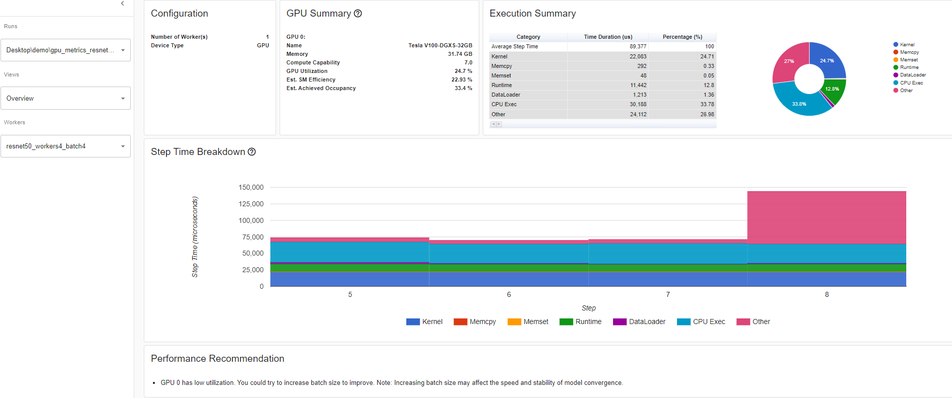
Overview details: Resnet50_batchsize4
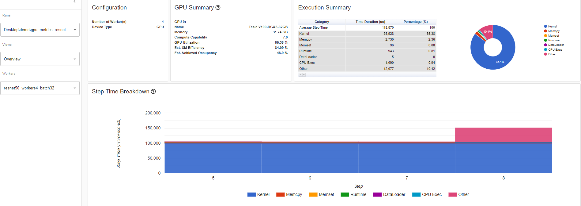
Overview details: Resnet50_batchsize32
Kernel View The kernel has “Blocks per SM” and “Est. Achieved Occupancy” which is a great tool to compare model runs.
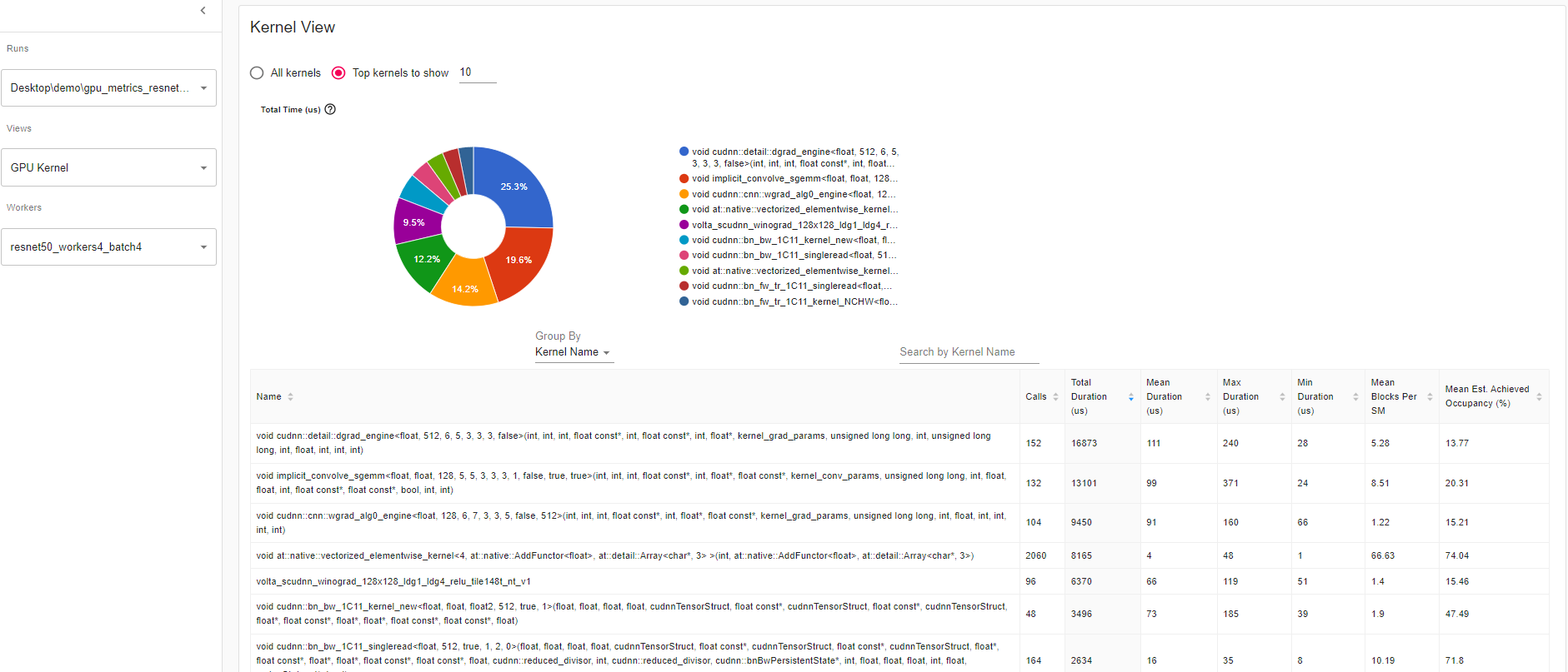
Mean Blocks per SM:
Blocks per SM = Blocks of this kernel / SM number of this GPU. If this number is less than 1, it indicates the GPU multiprocessors are not fully utilized. “Mean Blocks per SM” is weighted average of all runs of this kernel name, using each run’s duration as weight.
Mean Est. Achieved Occupancy:
Est. Achieved Occupancy is defined as above in overview. “Mean Est. Achieved Occupancy” is weighted average of all runs of this kernel name, using each run’s duration as weight.
Trace View This trace view displays a timeline that shows the duration of operators in your model and which system executed the operation. This view can help you identify whether the high consumption and long execution is because of input or model training. Currently, this trace view shows GPU Utilization and Est. SM Efficiency on a timeline.
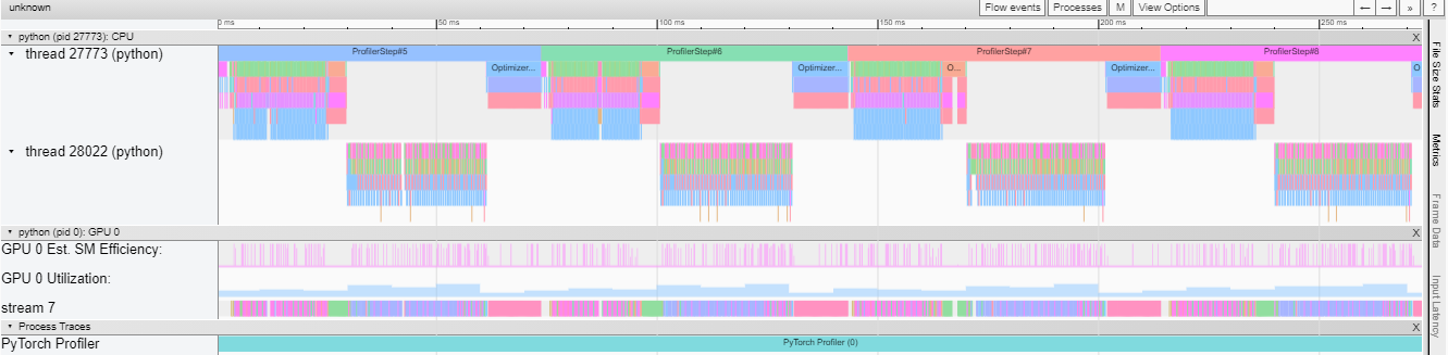
GPU utilization is calculated independently and divided into multiple 10 millisecond buckets. The buckets’ GPU utilization values are drawn alongside the timeline between 0 – 100%. In the above example, the “ProfilerStep5” GPU utilization during thread 28022’s busy time is higher than the following the one during “Optimizer.step”. This is where you can zoom-in to investigate why that is.
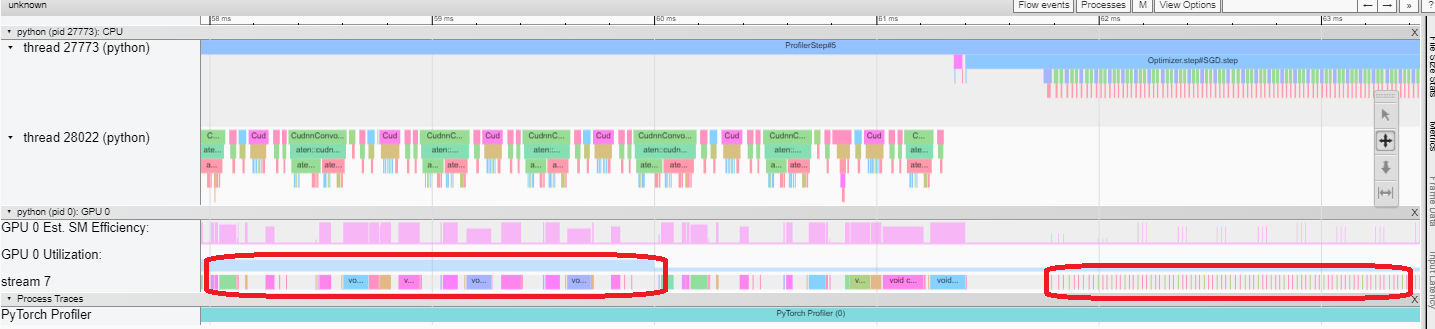
From above, we can see the former’s kernels are longer than the later’s kernels. The later’s kernels are too short in execution, which results in lower GPU utilization.
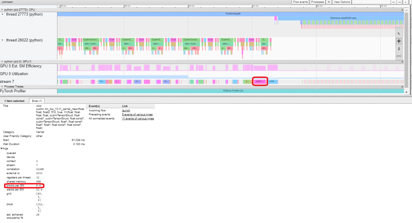
Est. SM Efficiency: Each kernel has a calculated est. SM efficiency between 0 – 100%. For example, the below kernel has only 64 blocks, while the SMs in this GPU is 80. Then its “Est. SM Efficiency” is 64/80, which is 0.8.
Cloud Storage Support
After running pip install tensorboard, to have data be read through these cloud providers, you can now run:
torch-tb-profiler[blob]
torch-tb-profiler[gs]
torch-tb-profiler[s3]
pip install torch-tb-profiler[blob], pip install torch-tb-profiler[gs], or pip install torch-tb-profiler[S3] to have data be read through these cloud providers. For more information, please refer to this README.
Jump to Source Code:
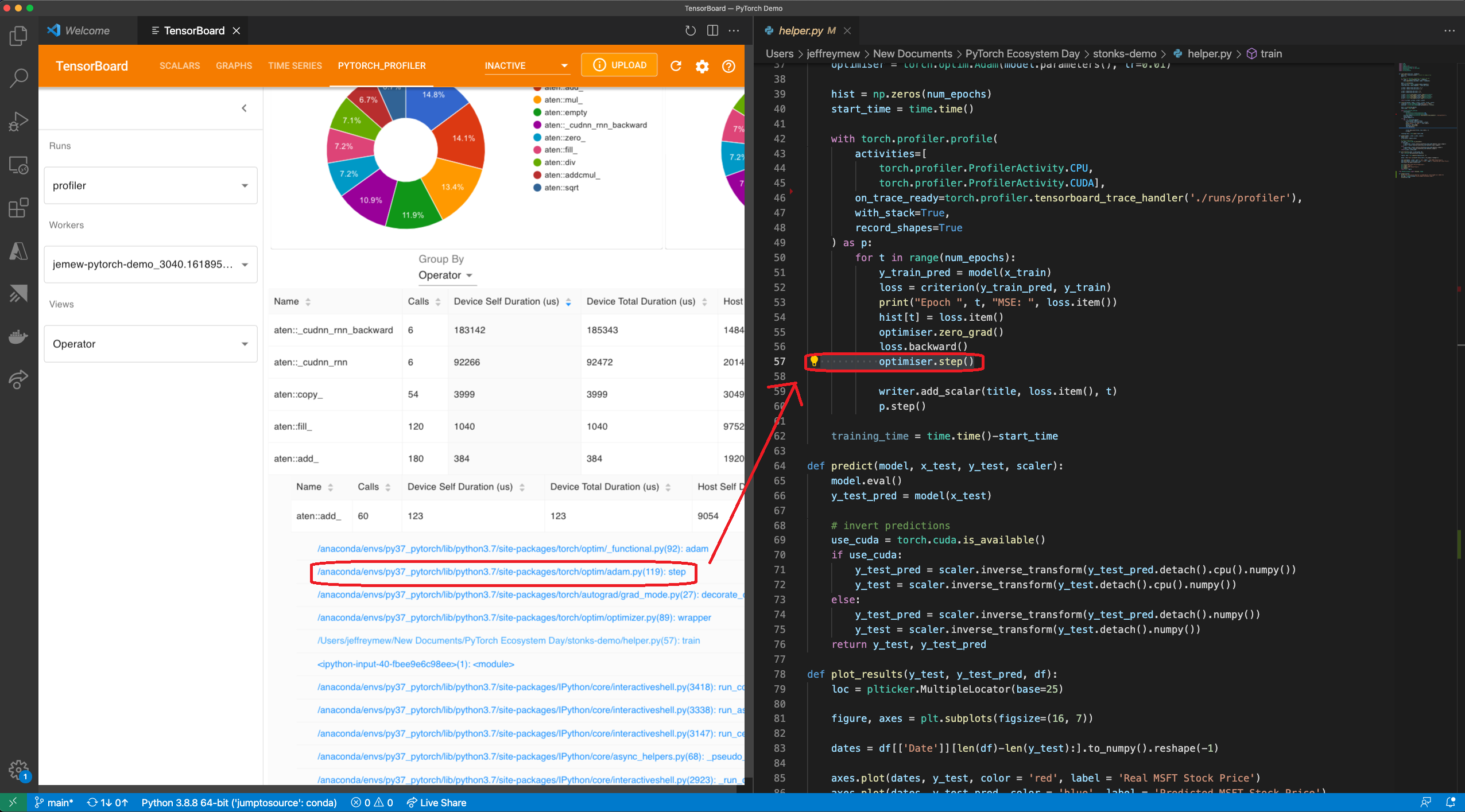
One of the great benefits of having both TensorBoard and the PyTorch Profiler being integrated directly in Visual Studio Code (VS Code) is the ability to directly jump to the source code (file and line) from the profiler stack traces. VS Code Python Extension now supports TensorBoard Integration.
Jump to source is ONLY available when Tensorboard is launched within VS Code. Stack tracing will appear on the plugin UI if the profiling with_stack=True. When you click on a stack trace from the PyTorch Profiler, VS Code will automatically open the corresponding file side by side and jump directly to the line of code of interest for you to debug. This allows you to quickly make actionable optimizations and changes to your code based on the profiling results and suggestions.
Gify: Jump to Source using Visual Studio Code Plug In UI
For how to optimize batch size performance, check out the step-by-step tutorial here. PyTorch Profiler is also integrated with PyTorch Lightning and you can simply launch your lightning training jobs with –trainer.profiler=pytorch flag to generate the traces.
What’s Next for the PyTorch Profiler?
You just saw how PyTorch Profiler can help optimize a model. You can now try the Profiler by pip install torch-tb-profiler to optimize your PyTorch model.
Look out for an advanced version of this tutorial in the future. We are also thrilled to continue to bring state-of-the-art tool to PyTorch users to improve ML performance. We’d love to hear from you. Feel free to open an issue here.
For new and exciting features coming up with PyTorch Profiler, follow @PyTorch on Twitter and check us out on pytorch.org.
Acknowledgements
The author would like to thank the contributions of the following individuals to this piece. From the Facebook side: Geeta Chauhan, Gisle Dankel, Woo Kim, Sam Farahzad, and Mark Saroufim. On the Microsoft side: AI Framework engineers (Teng Gao, Mike Guo, and Yang Gu), Guoliang Hua, and Thuy Nguyen.