1. Introduction
PyTorch supports two execution modes [1]: eager mode and graph mode. In eager mode, operators in a model are immediately executed as they are encountered. In contrast, in graph mode, operators are first synthesized into a graph, which will then be compiled and executed as a whole. Eager mode is easier to use, more suitable for ML researchers, and hence is the default mode of execution. On the other hand, graph mode typically delivers higher performance and hence is heavily used in production.
Specifically, graph mode enables operator fusion [2], wherein one operator is merged with another to reduce/localize memory reads as well as total kernel launch overhead. Fusion can be horizontal—taking a single operation (e.g., BatchNorm) that is independently applied to many operands and merging those operands into an array; and vertical—merging a kernel with another kernel that consumes the output of the first kernel (e.g., Convolution followed by ReLU).
Torch.FX [3, 4] (abbreviated as FX) is a publicly available toolkit as part of the PyTorch package that supports graph mode execution. In particular, it (1) captures the graph from a PyTorch program and (2) allows developers to write transformations on the captured graph. It is used inside Meta to optimize the training throughput of production models. By introducing a number of FX-based optimizations developed at Meta, we demonstrate the approach of using graph transformation to optimize PyTorch’s performance for production.
2. Background
Embedding tables are ubiquitous in recommendation systems. Section 3 will discuss three FX transformations that optimize accesses to embedding tables. In this section, we provide some background on FX (Section 2.1) and embedding tables (Section 2.2).
2.1 FX
Figure 1 is a simple example adopted from [3] which illustrates using FX to transform a PyTorch program. It contains three steps: (1) capturing the graph from a program, (2) modifying the graph (in this example, all uses of RELU are replaced by GELU), and (3) generating a new program from the modified graph.
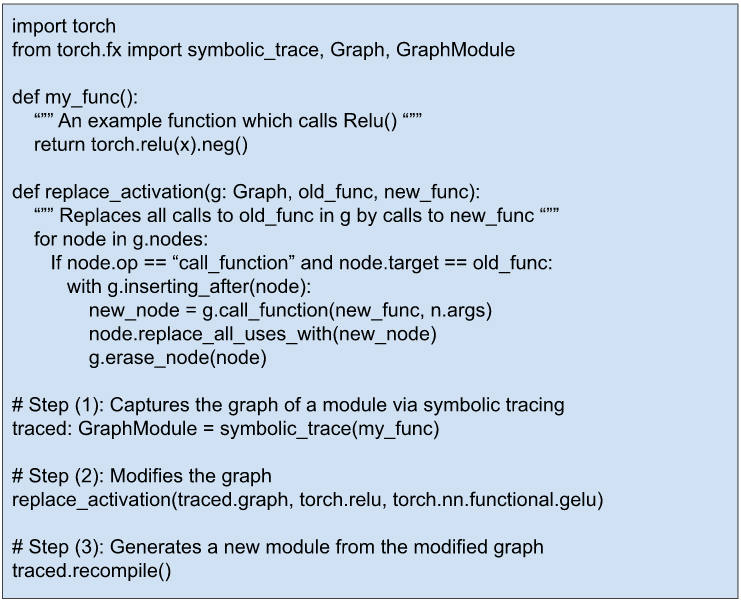
Figure 1: A FX example which replaces all uses of RELU by GELU in a PyTorch module.
The FX API [4] provides many more functionalities for inspecting and transforming PyTorch program graphs.
2.2 Embedding Tables
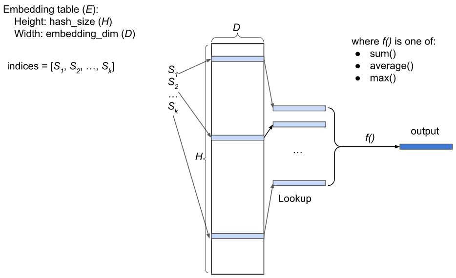
Figure 2: Illustration of an embedding table for a sparse feature with batch size = 1
In a recommendation system, sparse features (e.g., User ID, Story ID) are represented by embedding tables. An embedding table E is an HxD matrix, where H is the hash size, D is the embedding dimension. Each row of E is a vector of floats. Feature hashing [5] is used to map a sparse feature to a list of indices to E, say [S1,S2, …, Sk], where 0<=Si<H. Its output value is computed as f(E[S1], E[S2], …, E[Sk]), where E[Si] is the vector at row Si, and f is called the pooling function, which is typically one of the following functions: sum, average, maximum. See Figure 2 for an illustration.
To fully utilize the GPU, sparse features are usually processed in a batch. Each entity in a batch has its own list of indices. If a batch has B entities, a naive representation has B lists of indices. A more compact representation is to combine the B lists of indices into a single list of indices and add a list of the lengths of indices (one length for each entity in the batch). For example, if a batch has 3 entities whose lists of indices are as follows:
- Entity 1: indices = [10, 20]
- Entity 2: indices = [5, 9, 77, 81]
- Entity 3: indices = [15, 20, 45]
Then the indices and lengths for the entire batch will be:
- Indices = [10, 20, 5, 9, 77, 81, 15, 20, 45]
- Lengths = [2, 4, 3]
And the output of the embedding table lookup for the whole batch is a BxD matrix.
3. Three FX Transformations
We have developed three FX transformations that accelerate accesses to embedding tables. Section 3.1 discusses a transformation that combines multiple small input tensors into a single big tensor; Section 3.2 a transformation that fuses multiple, parallel compute chains into a single compute chain; and Section 3.3 a transformation that overlaps communication with computation.
3.1 Combining Input Sparse Features
Recall that an input sparse feature in a batch is represented by two lists: a list of indices and a list of B lengths, where B is the batch size. In PyTorch, these two lists are implemented as two tensors. When a PyTorch model is run on a GPU, embedding tables are commonly stored in the GPU memory (which is closer to the GPU and has much higher read/write bandwidth than the CPU memory). To use an input sparse feature, its two tensors need to be first copied from CPU to GPU. Nevertheless, per host-to-device memory copying requires a kernel launch, which is relatively expensive compared to the actual data transfer time. If a model uses many input sparse features, this copying could become a performance bottleneck (e.g., 1000 input sparse features would require copying 2000 tensors from host to device).
An optimization that reduces the number of host-to-device memcpy is to combine multiple input sparse features before sending them to the device. For instance, given the following three input features:
- Feature_A: indices = [106, 211, 7], lengths = [2, 1]
- Feature_B: indices = [52, 498, 616, 870, 1013], lengths = [3, 2]
- Feature_C: indices = [2011, 19, 351, 790], lengths = [1, 3]
The combined form is:
- Features_A_B_C: indices = [106, 211, 7, 52, 498, 616, 870, 1013, 2011, 19, 351, 790], lengths = [2, 1, 3, 2, 1, 3]
So, instead of copying 3×2=6 tensors from host to device, we only need to copy 2 tensors.
Figure 3(b) describes an implementation of this optimization, which has two components:
- On the CPU side: The input pipeline is modified to combine all the indices of sparse features into a single tensor and similarly all the lengths into another tensor. Then the two tensors are copied to the GPU.
- On the GPU side: Using FX, we insert a Permute_and_Split op into the model graph to recover the indices and lengths tensors of individual features from the combined tensors, and route them to the corresponding nodes downstream.
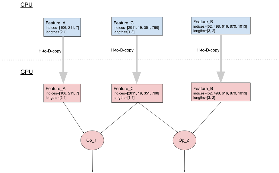
(a). Without the optimization
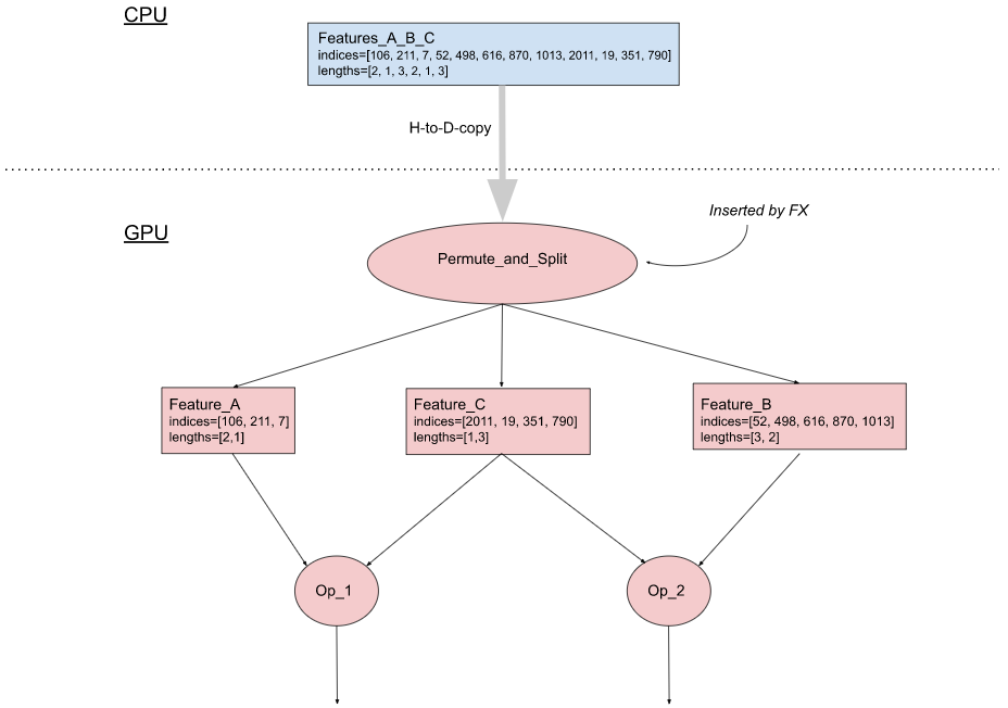
(b). With the optimization
Figure 3: Combining input sparse features
3.2 Horizontal fusion of computation chains started with accesses to embedding tables
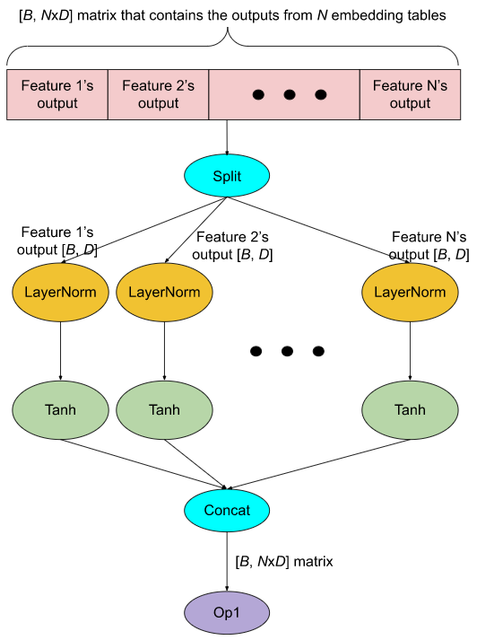
In a production model, it is fairly common to have 10s of embedding tables residing on each GPU. For performance reasons, lookups to these tables are grouped together so that their outputs are concatenated in a single big tensor (see the red part in Figure 4(a)). To apply computations to individual feature outputs, a Split op is used to divide the big tensors into N smaller tensors (where N is the number of features) and then the desired computations are applied to each tensor. This is shown in Figure 4(a), where the computation applied to each feature output O is Tanh(LayerNorm(O)). All the computation results are concatenated back to a big tensor, which is then passed to downstream ops (Op1 in Figure 4(a)).
The main runtime cost here is the GPU kernel launch overhead. For instance, the number of GPU kernel launches in Figure 4(a) is 2*N + 3 (each oval in the figure is a GPU kernel). This could become a performance issue because execution times of LayerNorm and Tanh on the GPU are short compared to their kernel launch times. In addition, the Split op may create an extra copy of the embedding output tensor, consuming additional GPU memory.
We use FX to implement an optimization called horizontal fusion which dramatically reduces the number of GPU kernel launches (in this example, the optimized number of GPU kernel launches is 5, see Figure 4(b)). Instead of doing an explicit Split, we use the Add_middle_dim op to reshape the 2D embedding tensor of shape (B, NxD) to a 3D tensor of shape (B, N, D). Then a single LayerNorm is applied to the last dimension of it. Then a single Tanh is applied to the result of the LayerNorm. At the end, we use the Remove_middle_dim op to reshape the Tanh’s result back to a 2D tensor. In addition, since Add_middle_dim and Remove_middle_dim only reshape the tensor without creating an extra copy, the amount of GPU memory consumption could be reduced as well.
(a). Without the optimization
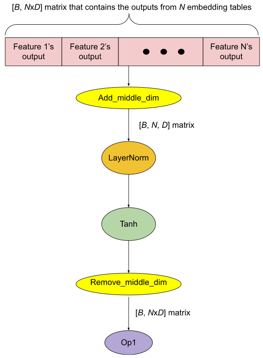
(b). With the optimization
Figure 4: Horizontal fusion
3.3 Overlapping Computation with Communication
Training of a production recommendation model is typically done on a distributed GPU system. Since the capacity of the device memory per GPU is not big enough to hold all the embedding tables in the model, they need to be distributed among the GPUs.
Within a training step, a GPU needs to read/write feature values from/to the embedding tables on the other GPUs. This is known as all-to-all communication [6] and can be a major performance bottleneck.
We use FX to implement a transformation that can overlap computation with all-to-all communication. Figure 5(a) shows the example of a model graph which has embedding table accesses (EmbeddingAllToAll) and other ops. Without any optimization, they are sequentially executed on a GPU stream, as shown in Figure 5(b). Using FX, we break EmbeddingAllToAll into EmbeddingAllToAll_Request and EmbeddingAllToAll_Wait, and schedule independent ops in between them.
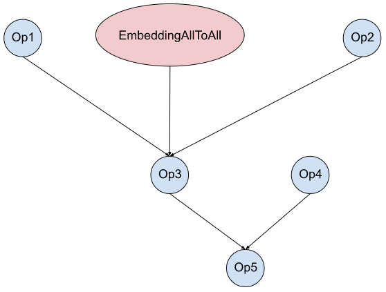
(a) Model graph
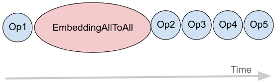
(b) Original execution order
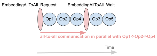
(c)Optimized execution order
Figure 5: Overlapping Computation with Communication
3.4 Summary
Table 1 summarizes the optimizations discussed in this section and the corresponding performance bottlenecks addressed.
| Optimization | Performance Bottleneck Addressed |
| Combining Input Sparse Features | Host-to-device memory copy |
| Horizontal fusion | GPU kernel launch overhead |
| Overlapping Computation with Communication | Embedding all-to-all access time |
Table 1: Summary of the optimizations and the performance bottlenecks addressed
We have also developed other FX transformations which are not discussed in this section due to space limitations.
To discover which models would benefit from these transformations, we analyzed the performance data collected by MAIProf [7] from the models that run at Meta’s data centers. Altogether, these transformations provide up to 2-3x of speedups compared to eager mode on a set of production models.
4. Concluding Remarks
The graph mode in PyTorch is preferred over the eager mode for production use for performance reasons. FX is a powerful tool for capturing and optimizing the graph of a PyTorch program. We demonstrate three FX transformations that are used to optimize production recommendation models inside Meta. We hope that this blog can motivate other PyTorch model developers to use graph transformations to boost their models’ performance.
References
[1] End-to-end Machine Learning Framework
[2] DNNFusion: Accelerating Deep Neural Networks Execution with Advanced Operator Fusion
[3] Torch.FX: Practical Program Capture and Transformation for Deep Learning In Python, MLSys 2022.
[4] Torch.fx—PyTorch 1.12 documentation
[5] Feature Hashing for Large Scale Multitask Learning
[6] NVIDIA Collective Communication Library Documentation
[7] Performance Debugging of Production PyTorch Models at Meta