TL;DR: PyTorch 2.0 nightly offers out-of-the-box performance improvement for Generative Diffusion models by using the new torch.compile() compiler and optimized implementations of Multihead Attention integrated with PyTorch 2.
Introduction
A large part of the recent progress in Generative AI came from denoising diffusion models, which allow producing high quality images and videos from text prompts. This family includes Imagen, DALLE, Latent Diffusion, and others. However, all models in this family share a common drawback: generation is rather slow, due to the iterative nature of the sampling process by which the images are produced. This makes it important to optimize the code running inside the sampling loop.
We took an open source implementation of a popular text-to-image diffusion model as a starting point and accelerated its generation using two optimizations available in PyTorch 2: compilation and fast attention implementation. Together with a few minor memory processing improvements in the code these optimizations give up to 49% inference speedup relative to the original implementation without xFormers, and 39% inference speedup relative to using the original code with xFormers (excluding the compilation time), depending on the GPU architecture and batch size. Importantly, the speedup comes without a need to install xFormers or any other extra dependencies.
The table below shows the improvement in runtime between the original implementation with xFormers installed and our optimized version with PyTorch-integrated memory efficient attention (originally developed for and released in the xFormers library) and PyTorch compilation. The compilation time is excluded.
Runtime improvement in % compared to original+xFormers
See the absolute runtime numbers in section “Benchmarking setup and results summary”
| GPU | Batch size 1 | Batch size 2 | Batch size 4 |
| P100 (no compilation) | -3.8 | 0.44 | 5.47 |
| T4 | 2.12 | 10.51 | 14.2 |
| A10 | -2.34 | 8.99 | 10.57 |
| V100 | 18.63 | 6.39 | 10.43 |
| A100 | 38.5 | 20.33 | 12.17 |
One can notice the following:
- The improvements are significant for powerful GPUs like A100 and V100. For those GPUs the improvement is most pronounced for batch size 1
- For less powerful GPUs we observe smaller speedups (or in two cases slight regressions). The batch size trend is reversed here: improvement is larger for larger batches
In the following sections we describe the applied optimizations and provide detailed benchmarking data, comparing the generation time with various optimization features on/off.
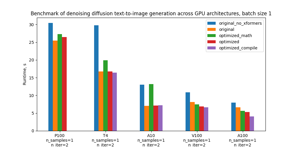
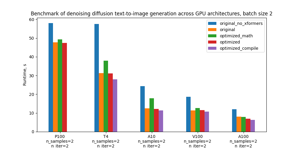
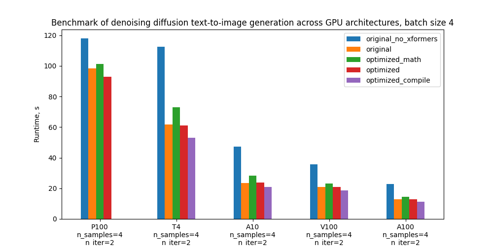
Specifically, we benchmark 5 configurations and the plots below compare their absolute performance for different GPUs and batch sizes. For definitions of these configurations see section “Benchmarking setup and results”.
Optimizations
Here we’ll go into more detail about the optimizations introduced into the model code. These optimizations rely on features of PyTorch 2.0 which has been released recently.
Optimized Attention
One part of the code which we optimized is the scaled dot-product attention. Attention is known to be a heavy operation: naive implementation materializes the attention matrix, leading to time and memory complexity quadratic in sequence length. It is common for diffusion models to use attention (CrossAttention) as part of Transformer blocks in multiple parts of the U-Net. Since the U-Net runs at every sampling step, this becomes a critical point to optimize. Instead of custom attention implementation one can use torch.nn.MultiheadAttention, which in PyTorch 2 has optimized attention implementation is integrated into it. This optimization schematically boils down to the following pseudocode:
class CrossAttention(nn.Module):
    def __init__(self, ...):
        # Create matrices: Q, K, V, out_proj
        ...
    def forward(self, x, context=None, mask=None):
       # Compute out = SoftMax(Q*K/sqrt(d))V
       # Return out_proj(out)
       …
gets replaced with
class CrossAttention(nn.Module):
    def __init__(self, ...):
        self.mha = nn.MultiheadAttention(...)
    def forward(self, x, context):
	return self.mha(x, context, context)
The optimized implementation of attention was available already in PyTorch 1.13 (see here) and widely adopted (see e.g. HuggingFace transformers library example). In particular, it integrates memory-efficient attention from the xFormers library and flash attention from https://arxiv.org/abs/2205.14135. PyTorch 2.0 expands this to additional attention functions such as cross attention and custom kernels for further acceleration, making it applicable to diffusion models.
Flash attention is available on GPUs with compute capability SM 7.5 or SM 8.x – for example, on T4, A10, and A100, which are included in our benchmark (you can check compute capability of each NVIDIA GPU here). However, in our tests on A100 the memory efficient attention performed better than flash attention for the particular case of diffusion models, due to the small number of attention heads and small batch size. PyTorch understands this and in this case chooses memory efficient attention over flash attention when both are available (see the logic here). For full control over the attention backends (memory-efficient attention, flash attention, “vanilla math”, or any future ones), power users can enable and disable them manually with the help of the context manager torch.backends.cuda.sdp_kernel.
Compilation
Compilation is a new feature of PyTorch 2.0, enabling significant speedups with a very simple user experience. To invoke the default behavior, simply wrap a PyTorch module or a function into torch.compile:
model = torch.compile(model)
PyTorch compiler then turns Python code into a set of instructions which can be executed efficiently without Python overhead. The compilation happens dynamically the first time the code is executed. With the default behavior, under the hood PyTorch utilized TorchDynamo to compile the code and TorchInductor to further optimize it. See this tutorial for more details.
Although the one-liner above is enough for compilation, certain modifications in the code can squeeze a larger speedup. In particular, one should avoid so-called graph breaks – places in the code which PyTorch can’t compile. As opposed to previous PyTorch compilation approaches (like TorchScript), PyTorch 2 compiler doesn’t break in this case. Instead it falls back on eager execution – so the code runs, but with reduced performance. We introduced a few minor changes to the model code to get rid of graph breaks. This included eliminating functions from libraries not supported by the compiler, such as inspect.isfunction and einops.rearrange. See this doc to learn more about graph breaks and how to eliminate them.
Theoretically, one can apply torch.compile on the whole diffusion sampling loop. However, in practice it is enough to just compile the U-Net. The reason is that torch.compile doesn’t yet have a loop analyzer and would recompile the code for each iteration of the sampling loop. Moreover, compiled sampler code is likely to generate graph breaks – so one would need to adjust it if one wants to get a good performance from the compiled version.
Note that compilation requires GPU compute capability >= SM 7.0 to run in non-eager mode. This covers all GPUs in our benchmarks – T4, V100, A10, A100 – except for P100 (see the full list).
Other optimizations
In addition, we have improved efficiency of GPU memory operations by eliminating some common pitfalls, e.g. creating a tensor on GPU directly rather than creating it on CPU and later moving to GPU. The places where such optimizations were necessary were determined by line-profiling and looking at CPU/GPU traces and Flame Graphs.
Benchmarking setup and results summary
We have two versions of code to compare: original and optimized. On top of this, several optimization features (xFormers, PyTorch memory efficient attention, compilation) can be turned on/off. Overall, as mentioned in the introduction, we will be benchmarking 5 configurations:
- Original code without xFormers
- Original code with xFormers
- Optimized code with vanilla math attention backend and no compilation
- Optimized code with memory-efficient attention backend and no compilation
- Optimized code with memory-efficient attention backend and compilation
As the original version we took the version of the code which uses PyTorch 1.12 and a custom implementation of attention. The optimized version uses nn.MultiheadAttention in CrossAttention and PyTorch 2.0.0.dev20230111+cu117. It also has a few other minor optimizations in PyTorch-related code.
The table below shows runtime of each version of the code in seconds, and the percentage improvement compared to the _original with xFormers. _The compilation time is excluded.
Runtimes for batch size 1. In parenthesis – relative improvement with respect to the “Original with xFormers” row
| Configuration | P100 | T4 | A10 | V100 | A100 |
| Original without xFormers | 30.4s (-19.3%) | 29.8s (-77.3%) | 13.0s (-83.9%) | 10.9s (-33.1%) | 8.0s (-19.3%) |
| Original with xFormers | 25.5s (0.0%) | 16.8s (0.0%) | 7.1s (0.0%) | 8.2s (0.0%) | 6.7s (0.0%) |
| Optimized with vanilla math attention, no compilation | 27.3s (-7.0%) | 19.9s (-18.7%) | 13.2s (-87.2%) | 7.5s (8.7%) | 5.7s (15.1%) |
| Optimized with mem. efficient attention, no compilation | 26.5s (-3.8%) | 16.8s (0.2%) | 7.1s (-0.8%) | 6.9s (16.0%) | 5.3s (20.6%) |
| Optimized with mem. efficient attention and compilation | – | 16.4s (2.1%) | 7.2s (-2.3%) | 6.6s (18.6%) | 4.1s (38.5%) |
Runtimes for batch size 2
| Configuration | P100 | T4 | A10 | V100 | A100 |
| Original without xFormers | 58.0s (-21.6%) | 57.6s (-84.0%) | 24.4s (-95.2%) | 18.6s (-63.0%) | 12.0s (-50.6%) |
| Original with xFormers | 47.7s (0.0%) | 31.3s (0.0%) | 12.5s (0.0%) | 11.4s (0.0%) | 8.0s (0.0%) |
| Optimized with vanilla math attention, no compilation | 49.3s (-3.5%) | 37.9s (-21.0%) | 17.8s (-42.2%) | 12.7s (-10.7%) | 7.8s (1.8%) |
| Optimized with mem. efficient attention, no compilation | 47.5s (0.4%) | 31.2s (0.5%) | 12.2s (2.6%) | 11.5s (-0.7%) | 7.0s (12.6%) |
| Optimized with mem. efficient attention and compilation | – | 28.0s (10.5%) | 11.4s (9.0%) | 10.7s (6.4%) | 6.4s (20.3%) |
Runtimes for batch size 4
| Configuration | P100 | T4 | A10 | V100 | A100 |
| Original without xFormers | 117.9s (-20.0%) | 112.4s (-81.8%) | 47.2s (-101.7%) | 35.8s (-71.9%) | 22.8s (-78.9%) |
| Original with xFormers | 98.3s (0.0%) | 61.8s (0.0%) | 23.4s (0.0%) | 20.8s (0.0%) | 12.7s (0.0%) |
| Optimized with vanilla math attention, no compilation | 101.1s (-2.9%) | 73.0s (-18.0%) | 28.3s (-21.0%) | 23.3s (-11.9%) | 14.5s (-13.9%) |
| Optimized with mem. efficient attention, no compilation | 92.9s (5.5%) | 61.1s (1.2%) | 23.9s (-1.9%) | 20.8s (-0.1%) | 12.8s (-0.9%) |
| Optimized with mem. efficient attention and compilation | – | 53.1s (14.2%) | 20.9s (10.6%) | 18.6s (10.4%) | 11.2s (12.2%) |
To minimize fluctuations and external influence on the performance of the benchmarked code, we ran each version of the code one after another, and then repeated this sequence 10 times: A, B, C, D, E, A, B, … So the results of a typical run would look like the one in the picture below.. Note that one shouldn’t rely on comparison of absolute run times between different graphs, but comparison of run times_ inside_ one graph is pretty reliable, thanks to our benchmarking setup.
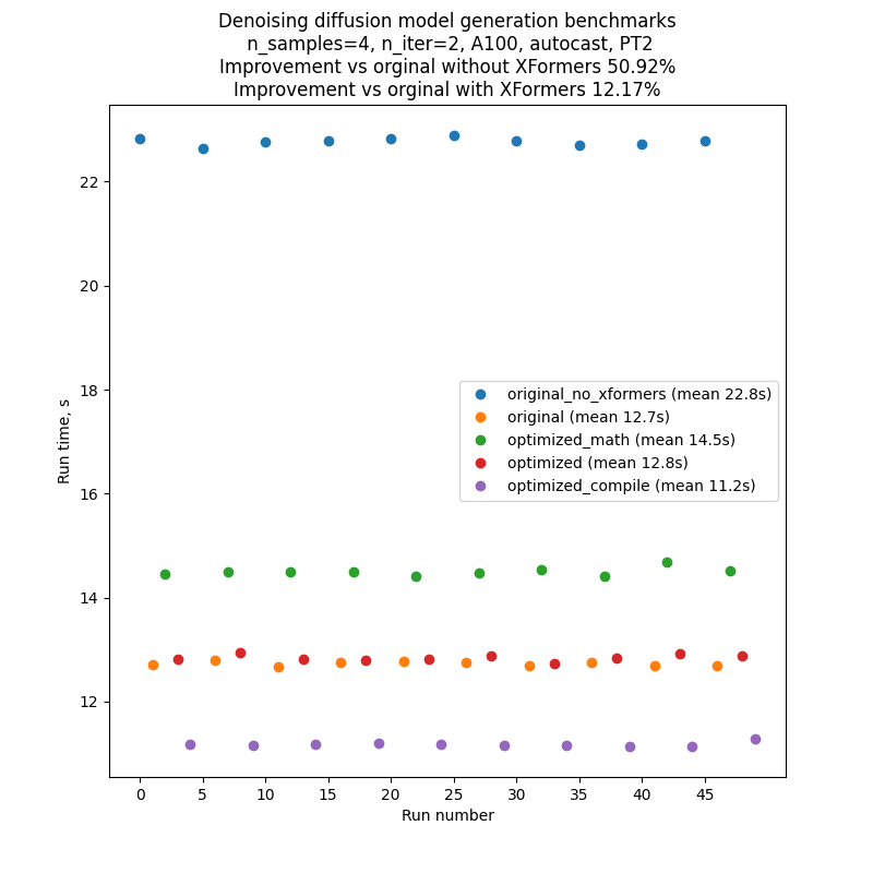
Each run of text-to-image generation script produces several batches, the number of which is regulated by the CLI parameter --n_iter. In the benchmarks we used n_iter = 2, but introduced an additional “warm-up” iteration, which doesn’t contribute to the run time. This was necessary for the runs with compilation, because compilation happens the first time the code runs, and so the first iteration is much longer than all subsequent. To make comparison fair, we also introduced this additional “warm-up” iteration to all other runs.
The numbers in the table above are for number of iterations 2 (plus a “warm-up one”), prompt ”A photo”, seed 1, PLMS sampler, and autocast turned on.
Benchmarks were done using P100, V100, A100, A10 and T4 GPUs. The T4 benchmarks were done in Google Colab Pro. The A10 benchmarks were done on g5.4xlarge AWS instances with 1 GPU.
Conclusions and next steps
We have shown that new features of PyTorch 2 – compiler and optimized attention implementation – give performance improvements exceeding or comparable with what previously required installation of an external dependency (xFormers). PyTorch achieved this, in particular, by integrating memory efficient attention from xFormers into its codebase. This is a significant improvement for user experience, given that xFormers, being a state-of-the-art library, in many scenarios requires custom installation process and long builds.
There are a few natural directions in which this work can be continued:
- The optimizations we implemented and described here are only benchmarked for text-to-image inference so far. It would be interesting to see how they affect training performance. PyTorch compilation can be directly applied to training; enabling training with PyTorch optimized attention is on the roadmap
- We intentionally minimized changes to the original model code. Further profiling and optimization can probably bring more improvements
- At the moment compilation is applied only to the U-Net model inside the sampler. Since there is a lot happening outside of U-Net (e.g. operations directly in the sampling loop), it would be beneficial to compile the whole sampler. However, this would require analysis of the compilation process to avoid recompilation at every sampling step
- Current code only applies compilation within the PLMS sampler, but it should be trivial to extend it to other samplers
- Besides text-to-image generation, diffusion models are also applied to other tasks – image-to-image and inpainting. It would be interesting to measure how their performance improves from PyTorch 2 optimizations
See if you can increase performance of open source diffusion models using the methods we described, and share the results!
Resources
- PyTorch 2.0 overview, which has a lot of information on
torch.compile:https://pytorch.org/get-started/pytorch-2.0/ - Tutorial on
torch.compile: https://pytorch.org/tutorials/intermediate/torch_compile_tutorial.html - General compilation troubleshooting: https://pytorch.org/docs/stable/torch.compiler_troubleshooting.html
- Details on graph breaks: https://pytorch.org/docs/stable/torch.compiler_faq.html#identifying-the-cause-of-a-graph-break
- Details on guards: https://pytorch.org/docs/stable/torch.compiler_guards_overview.html
- Video deep dive on TorchDynamo https://www.youtube.com/watch?v=egZB5Uxki0I
- Tutorial on optimized attention in PyTorch 1.12: https://pytorch.org/tutorials/beginner/bettertransformer_tutorial.html
Acknowledgements
We would like to thank Geeta Chauhan, Natalia Gimelshein, Patrick Labatut, Bert Maher, Mark Saroufim, Michael Voznesensky and Francisco Massa for their valuable advice and early feedback on the text.
Special thanks to Yudong Tao initiating the work on using PyTorch native attention in diffusion models.