Audio Feature Extractions

torchaudio implements feature extractions commonly used in the audio domain. They are available in torchaudio.functional and torchaudio.transforms.

functional implements features as standalone functions. They are stateless.

transforms implements features as objects, using implementations from functional and torch.nn.Module. Because all transforms are subclasses of torch.nn.Module, they can be serialized using TorchScript.

For the complete list of available features, please refer to the documentation. In this tutorial, we will look into converting between the time domain and frequency domain (Spectrogram, GriffinLim, MelSpectrogram).

# When running this tutorial in Google Colab, install the required packages
# with the following.
# !pip install torchaudio librosa

import torch
import torchaudio
import torchaudio.functional as F
import torchaudio.transforms as T

print(torch.__version__)
print(torchaudio.__version__)

Out:

1.11.0+cpu
0.11.0+cpu

Preparing data and utility functions (skip this section)

# @title Prepare data and utility functions. {display-mode: "form"}
# @markdown
# @markdown You do not need to look into this cell.
# @markdown Just execute once and you are good to go.
# @markdown
# @markdown In this tutorial, we will use a speech data from [VOiCES dataset](https://iqtlabs.github.io/voices/),
# @markdown which is licensed under Creative Commos BY 4.0.

# -------------------------------------------------------------------------------
# Preparation of data and helper functions.
# -------------------------------------------------------------------------------

import os

import librosa
import matplotlib.pyplot as plt
import requests
from IPython.display import Audio, display


_SAMPLE_DIR = "_assets"

SAMPLE_WAV_SPEECH_URL = "https://pytorch-tutorial-assets.s3.amazonaws.com/VOiCES_devkit/source-16k/train/sp0307/Lab41-SRI-VOiCES-src-sp0307-ch127535-sg0042.wav"  # noqa: E501
SAMPLE_WAV_SPEECH_PATH = os.path.join(_SAMPLE_DIR, "speech.wav")

os.makedirs(_SAMPLE_DIR, exist_ok=True)


def _fetch_data():
    uri = [
        (SAMPLE_WAV_SPEECH_URL, SAMPLE_WAV_SPEECH_PATH),
    ]
    for url, path in uri:
        with open(path, "wb") as file_:
            file_.write(requests.get(url).content)


_fetch_data()


def _get_sample(path, resample=None):
    effects = [["remix", "1"]]
    if resample:
        effects.extend(
            [
                ["lowpass", f"{resample // 2}"],
                ["rate", f"{resample}"],
            ]
        )
    return torchaudio.sox_effects.apply_effects_file(path, effects=effects)


def get_speech_sample(*, resample=None):
    return _get_sample(SAMPLE_WAV_SPEECH_PATH, resample=resample)


def print_stats(waveform, sample_rate=None, src=None):
    if src:
        print("-" * 10)
        print("Source:", src)
        print("-" * 10)
    if sample_rate:
        print("Sample Rate:", sample_rate)
    print("Shape:", tuple(waveform.shape))
    print("Dtype:", waveform.dtype)
    print(f" - Max:     {waveform.max().item():6.3f}")
    print(f" - Min:     {waveform.min().item():6.3f}")
    print(f" - Mean:    {waveform.mean().item():6.3f}")
    print(f" - Std Dev: {waveform.std().item():6.3f}")
    print()
    print(waveform)
    print()


def plot_spectrogram(spec, title=None, ylabel="freq_bin", aspect="auto", xmax=None):
    fig, axs = plt.subplots(1, 1)
    axs.set_title(title or "Spectrogram (db)")
    axs.set_ylabel(ylabel)
    axs.set_xlabel("frame")
    im = axs.imshow(librosa.power_to_db(spec), origin="lower", aspect=aspect)
    if xmax:
        axs.set_xlim((0, xmax))
    fig.colorbar(im, ax=axs)
    plt.show(block=False)


def plot_waveform(waveform, sample_rate, title="Waveform", xlim=None, ylim=None):
    waveform = waveform.numpy()

    num_channels, num_frames = waveform.shape
    time_axis = torch.arange(0, num_frames) / sample_rate

    figure, axes = plt.subplots(num_channels, 1)
    if num_channels == 1:
        axes = [axes]
    for c in range(num_channels):
        axes[c].plot(time_axis, waveform[c], linewidth=1)
        axes[c].grid(True)
        if num_channels > 1:
            axes[c].set_ylabel(f"Channel {c+1}")
        if xlim:
            axes[c].set_xlim(xlim)
        if ylim:
            axes[c].set_ylim(ylim)
    figure.suptitle(title)
    plt.show(block=False)


def play_audio(waveform, sample_rate):
    waveform = waveform.numpy()

    num_channels, num_frames = waveform.shape
    if num_channels == 1:
        display(Audio(waveform[0], rate=sample_rate))
    elif num_channels == 2:
        display(Audio((waveform[0], waveform[1]), rate=sample_rate))
    else:
        raise ValueError("Waveform with more than 2 channels are not supported.")


def plot_mel_fbank(fbank, title=None):
    fig, axs = plt.subplots(1, 1)
    axs.set_title(title or "Filter bank")
    axs.imshow(fbank, aspect="auto")
    axs.set_ylabel("frequency bin")
    axs.set_xlabel("mel bin")
    plt.show(block=False)


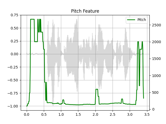
def plot_pitch(waveform, sample_rate, pitch):
    figure, axis = plt.subplots(1, 1)
    axis.set_title("Pitch Feature")
    axis.grid(True)

    end_time = waveform.shape[1] / sample_rate
    time_axis = torch.linspace(0, end_time, waveform.shape[1])
    axis.plot(time_axis, waveform[0], linewidth=1, color="gray", alpha=0.3)

    axis2 = axis.twinx()
    time_axis = torch.linspace(0, end_time, pitch.shape[1])
    axis2.plot(time_axis, pitch[0], linewidth=2, label="Pitch", color="green")

    axis2.legend(loc=0)
    plt.show(block=False)


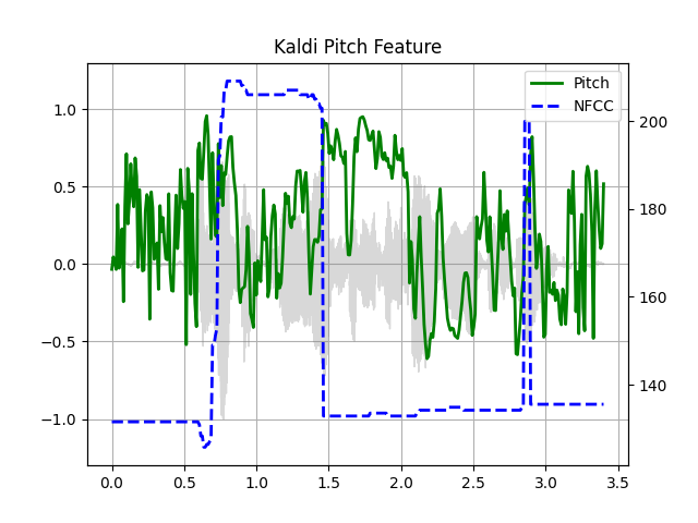
def plot_kaldi_pitch(waveform, sample_rate, pitch, nfcc):
    figure, axis = plt.subplots(1, 1)
    axis.set_title("Kaldi Pitch Feature")
    axis.grid(True)

    end_time = waveform.shape[1] / sample_rate
    time_axis = torch.linspace(0, end_time, waveform.shape[1])
    axis.plot(time_axis, waveform[0], linewidth=1, color="gray", alpha=0.3)

    time_axis = torch.linspace(0, end_time, pitch.shape[1])
    ln1 = axis.plot(time_axis, pitch[0], linewidth=2, label="Pitch", color="green")
    axis.set_ylim((-1.3, 1.3))

    axis2 = axis.twinx()
    time_axis = torch.linspace(0, end_time, nfcc.shape[1])
    ln2 = axis2.plot(time_axis, nfcc[0], linewidth=2, label="NFCC", color="blue", linestyle="--")

    lns = ln1 + ln2
    labels = [l.get_label() for l in lns]
    axis.legend(lns, labels, loc=0)
    plt.show(block=False)

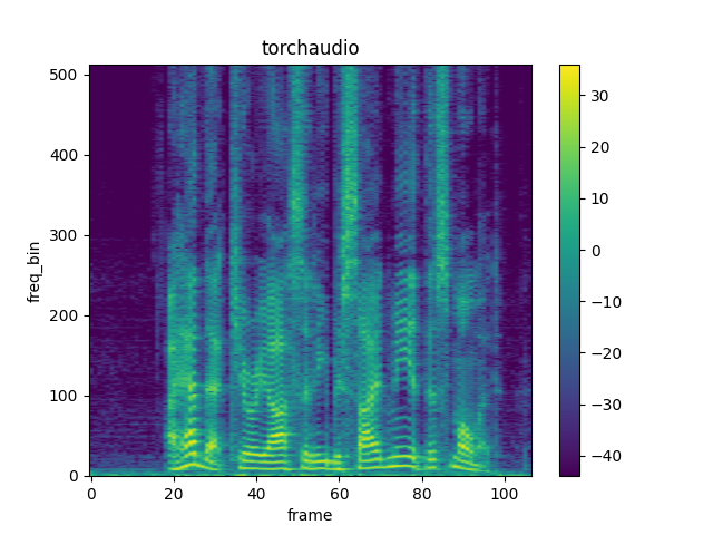
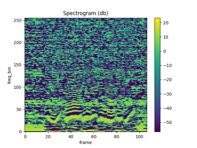
Spectrogram

To get the frequency make-up of an audio signal as it varies with time, you can use torchaudio.functional.Spectrogram().

waveform, sample_rate = get_speech_sample()

n_fft = 1024
win_length = None
hop_length = 512

# define transformation
spectrogram = T.Spectrogram(
    n_fft=n_fft,
    win_length=win_length,
    hop_length=hop_length,
    center=True,
    pad_mode="reflect",
    power=2.0,
)
# Perform transformation
spec = spectrogram(waveform)

print_stats(spec)
plot_spectrogram(spec[0], title="torchaudio")

Out:

Shape: (1, 513, 107)
Dtype: torch.float32
 - Max:     4000.533
 - Min:      0.000
 - Mean:     5.726
 - Std Dev: 70.301

tensor([[[7.8743e+00, 4.4462e+00, 5.6781e-01,  ..., 2.7694e+01,
          8.9546e+00, 4.1289e+00],
         [7.1094e+00, 3.2595e+00, 7.3520e-01,  ..., 1.7141e+01,
          4.4812e+00, 8.0840e-01],
         [3.8374e+00, 8.2490e-01, 3.0779e-01,  ..., 1.8502e+00,
          1.1777e-01, 1.2369e-01],
         ...,
         [3.4699e-07, 1.0605e-05, 1.2395e-05,  ..., 7.4096e-06,
          8.2065e-07, 1.0176e-05],
         [4.7173e-05, 4.4330e-07, 3.9445e-05,  ..., 3.0623e-05,
          3.9746e-07, 8.1572e-06],
         [1.3221e-04, 1.6440e-05, 7.2536e-05,  ..., 5.4662e-05,
          1.1663e-05, 2.5758e-06]]])

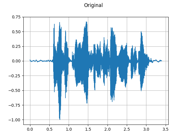
GriffinLim

To recover a waveform from a spectrogram, you can use GriffinLim.

torch.random.manual_seed(0)
waveform, sample_rate = get_speech_sample()
plot_waveform(waveform, sample_rate, title="Original")
play_audio(waveform, sample_rate)

n_fft = 1024
win_length = None
hop_length = 512

spec = T.Spectrogram(
    n_fft=n_fft,
    win_length=win_length,
    hop_length=hop_length,
)(waveform)

griffin_lim = T.GriffinLim(
    n_fft=n_fft,
    win_length=win_length,
    hop_length=hop_length,
)
waveform = griffin_lim(spec)

plot_waveform(waveform, sample_rate, title="Reconstructed")
play_audio(waveform, sample_rate)

• 
• 

Out:

<IPython.lib.display.Audio object>
<IPython.lib.display.Audio object>

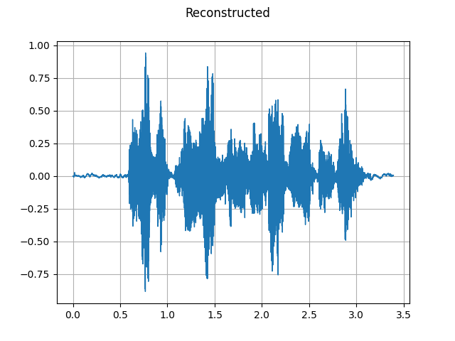
Mel Filter Bank

torchaudio.functional.melscale_fbanks() generates the filter bank for converting frequency bins to mel-scale bins.

Since this function does not require input audio/features, there is no equivalent transform in torchaudio.transforms().

n_fft = 256
n_mels = 64
sample_rate = 6000

mel_filters = F.melscale_fbanks(
    int(n_fft // 2 + 1),
    n_mels=n_mels,
    f_min=0.0,
    f_max=sample_rate / 2.0,
    sample_rate=sample_rate,
    norm="slaney",
)
plot_mel_fbank(mel_filters, "Mel Filter Bank - torchaudio")

Comparison against librosa

For reference, here is the equivalent way to get the mel filter bank with librosa.

mel_filters_librosa = librosa.filters.mel(
    sr=sample_rate,
    n_fft=n_fft,
    n_mels=n_mels,
    fmin=0.0,
    fmax=sample_rate / 2.0,
    norm="slaney",
    htk=True,
).T

plot_mel_fbank(mel_filters_librosa, "Mel Filter Bank - librosa")

mse = torch.square(mel_filters - mel_filters_librosa).mean().item()
print("Mean Square Difference: ", mse)

Out:

Mean Square Difference:  3.795462323290159e-17

MelSpectrogram

Generating a mel-scale spectrogram involves generating a spectrogram and performing mel-scale conversion. In torchaudio, torchaudio.transforms.MelSpectrogram() provides this functionality.

waveform, sample_rate = get_speech_sample()

n_fft = 1024
win_length = None
hop_length = 512
n_mels = 128

mel_spectrogram = T.MelSpectrogram(
    sample_rate=sample_rate,
    n_fft=n_fft,
    win_length=win_length,
    hop_length=hop_length,
    center=True,
    pad_mode="reflect",
    power=2.0,
    norm="slaney",
    onesided=True,
    n_mels=n_mels,
    mel_scale="htk",
)

melspec = mel_spectrogram(waveform)
plot_spectrogram(melspec[0], title="MelSpectrogram - torchaudio", ylabel="mel freq")

Comparison against librosa

For reference, here is the equivalent means of generating mel-scale spectrograms with librosa.

melspec_librosa = librosa.feature.melspectrogram(
    y=waveform.numpy()[0],
    sr=sample_rate,
    n_fft=n_fft,
    hop_length=hop_length,
    win_length=win_length,
    center=True,
    pad_mode="reflect",
    power=2.0,
    n_mels=n_mels,
    norm="slaney",
    htk=True,
)
plot_spectrogram(melspec_librosa, title="MelSpectrogram - librosa", ylabel="mel freq")

mse = torch.square(melspec - melspec_librosa).mean().item()
print("Mean Square Difference: ", mse)

Out:

Mean Square Difference:  1.1827383517015733e-10

MFCC

waveform, sample_rate = get_speech_sample()

n_fft = 2048
win_length = None
hop_length = 512
n_mels = 256
n_mfcc = 256

mfcc_transform = T.MFCC(
    sample_rate=sample_rate,
    n_mfcc=n_mfcc,
    melkwargs={
        "n_fft": n_fft,
        "n_mels": n_mels,
        "hop_length": hop_length,
        "mel_scale": "htk",
    },
)

mfcc = mfcc_transform(waveform)

plot_spectrogram(mfcc[0])

Comparing against librosa

melspec = librosa.feature.melspectrogram(
    y=waveform.numpy()[0],
    sr=sample_rate,
    n_fft=n_fft,
    win_length=win_length,
    hop_length=hop_length,
    n_mels=n_mels,
    htk=True,
    norm=None,
)

mfcc_librosa = librosa.feature.mfcc(
    S=librosa.core.spectrum.power_to_db(melspec),
    n_mfcc=n_mfcc,
    dct_type=2,
    norm="ortho",
)

plot_spectrogram(mfcc_librosa)

mse = torch.square(mfcc - mfcc_librosa).mean().item()
print("Mean Square Difference: ", mse)

Out:

Mean Square Difference:  1.0665760040283203

Pitch

waveform, sample_rate = get_speech_sample()

pitch = F.detect_pitch_frequency(waveform, sample_rate)
plot_pitch(waveform, sample_rate, pitch)
play_audio(waveform, sample_rate)

Out:

<IPython.lib.display.Audio object>

Kaldi Pitch (beta)

Kaldi Pitch feature [1] is a pitch detection mechanism tuned for automatic speech recognition (ASR) applications. This is a beta feature in torchaudio, and it is available as torchaudio.functional.compute_kaldi_pitch().

1. A pitch extraction algorithm tuned for automatic speech recognition

   Ghahremani, B. BabaAli, D. Povey, K. Riedhammer, J. Trmal and S. Khudanpur

   2014 IEEE International Conference on Acoustics, Speech and Signal Processing (ICASSP), Florence, 2014, pp. 2494-2498, doi: 10.1109/ICASSP.2014.6854049. [abstract], [paper]

waveform, sample_rate = get_speech_sample(resample=16000)

pitch_feature = F.compute_kaldi_pitch(waveform, sample_rate)
pitch, nfcc = pitch_feature[..., 0], pitch_feature[..., 1]

plot_kaldi_pitch(waveform, sample_rate, pitch, nfcc)
play_audio(waveform, sample_rate)

Out:

<IPython.lib.display.Audio object>