Recently, the PyTorch team released Helion, a new domain-specific and PyTorch-based language to make the development of high-performing but portable kernels easier. With extensive autotuning built in, Helion has the promise to move the forefront of performance portability further than Triton.
To test this promise (and learn Helion), we embarked on the challenge to write one of AI’s most performance-critical kernels in Helion: Paged Attention, the core of vLLM.
In the past year, we contributed a performance and platform portable attention backend for vLLM written entirely in Triton, which has no external dependencies and runs on NVIDIA, AMD, and Intel GPUs (see our PyTorch conference talk). Hence, we implemented one of the kernels (unified_attention_2d) in Helion as a new experimental backend in vLLM (PR#27293).
Brief Background to vLLM, Triton, and Helion
vLLM is widely used for LLM inference and part of the PyTorch Foundation. vLLM is increasingly being adopted in production and can be executed on NVIDIA, AMD, and Intel GPUs, as well as custom accelerators like Google’s TPU, Huawei’s Ascend NPU, AWS Inferentia, or IBM Spyre. vLLM features efficient and high-performance inference for nearly all LLM models, which is achieved by its well-designed software architecture and deep integration with torch.compile.
Triton is a domain-specific language (DSL) that can be written in Python and offers just-in-time (JIT) compilation to AMD, Intel, and NVIDIA GPUs. Triton kernels have shown to demonstrate state-of-the-art performance and can be portable. For example, we have written paged attention in Triton and the very same kernel code achieves state-of-the-art performance on NVIDIA H100 and AMD MI300 (you can read our extensive paper or the related blog post). For this we also leveraged Triton’s autotuner in a limited way. However, autotuning in Triton has severe limitations that prohibit its use in production, despite its positive impact on performance portability. Hence, for our Triton attention backend, we use simple if-else statements as heuristics for now.
Besides this, Triton is also the output language of PyTorch Inductor, the compile component of torch.compile.
Helion is yet another DSL, which became beta at the end of October. Helion considers itself as “tiled PyTorch” and has broadly two aims: First, to bring tiling to PyTorch so that tiled programs can be written using PyTorch APIs. And second, enhance portability by extensive autotuning. In contrast to Triton, Helion’s autotuner has not only a usable caching mechanism, but the autotuner also has a lot more degrees of freedom. This larger freedom comes from the fact that in Helion, the autotuner can also change algorithmic aspects of an implementation, in addition to lower-level compile flags like the number of warps or pipeline depths. It also features advanced search algorithms, which is something we previously investigated in the context of Triton.
Implementation Details: How to write Paged Attention in Tiled PyTorch
Launch Grid and approach of parallelization
As a starting point, we wanted to re-implement the simpler “2D” version of our unified attention Triton kernels. It is called “2D” because this kernel has a two-dimensional launch grid (see details here), and we selected this kernel version, since we thought the parallel tiled softmax implementation would be too complex in the beginning.
However, since launch grids are handled differently in Helion than Triton, we did not follow the 2D approach 1:1, but built a Helion kernel around the core concept of “Q blocks”. This concept is illustrated in the following Figure:

Figure 1: Concept of “Q blocks” in our Helion kernel.
In this Figure, we see the three dimensions of one request that need to be computed. An attention kernel needs to iterate over all the query tokens up to the query_length (bottom axis). In our kernel, we fetch multiple query tokens at the same time. This tile size, TILE_Q, is tuneable. Next, for each token, there are multiple query heads and KV-heads (left axis). We have re-implemented our QGA optimization so that all query heads for one KV head are fetched at once. The query-heads-per-kv-head (QpKV) is the tile size in this direction and is called TILE_M. Finally, we have to iterate over the KV cache for this query up to the current context length in tuneable blocks of size TILE_N (diagonal axis). In this inner loop, the actual attention computation, including matrix multiplications (hl.dot), is happening, using an online softmax implementation. In the kernel, there is an additional loop around all of this to iterate over all requests in a batch (not in the Figure).
However, the input tensor, as it is handled by vLLM, has as first dimension the number of sequences and the query length combined (which is often called “flattened varlen” layout). Consequently, vLLM provides an extra tensor that is used as an index to know which token belongs to which sequence.
Hence, after experimenting with some implementations, we settled on the four-loop approach described above:
# registering tunable block sizes
q_block_size = hl.register_block_size(1, q_block_padded_size)   num_pages_at_once = hl.register_block_size(1, 32)

# outer loop -> becomes the launch grid
for seq_tile, tile_m in hl.tile([num_seqs, num_query_heads],
      block_size=[1, num_queries_per_kv],):

    seq_len = t_seq_lens[seq_tile]
    query_start = t_query_start_lens[seq_tile]
    query_end = t_query_start_lens[seq_tile + 1]
    query_len = query_end - query_start

    # loop over the query of one request
    for tile_q in hl.tile(query_len, block_size=q_block_size):
    ...

       # loop over KV cache
        for tile_n in hl.tile(num_blocks,
              block_size=num_pages_at_once):

        ...
As can be seen, the outer loop is a fused loop and has two dimensions: The sequences in a batch and the QpKV. This outer loop will become the launch grid in Triton (Helion recommends to use hl.tile over hl.grid, also for the outer loop). Since we need the tuned block sizes also for e.g. boundary computation before the loop, we register the block sizes explicitly before. Additionally, to make the launch grid simpler, we changed the order of loops in the implementation vs. the description above and let the outer loop iterate over the query heads.
Next, the second loop is then over the query length of the selected sequence with a tuneable tile size. But please note that we pad the upper bound of this tile size (see q_block_padded_size), so that neither the JIT compiler nor the autotuner are triggered for all possible combinations of query lengths. Instead, we provide here only padded length to the power of two, which reduces the JIT/autotune overhead at runtime. The innermost loop is over the number of KV cache pages in the selected sequence. Hence, also the upper bound of the corresponding registered block size means 32 pages of KV cache memory (each of e.g. 16 tokens).
The Triton code generated by this could look like:
# src[helion_unified_attention.py:129]: for seq_tile, tile_m in hl.tile(
# src[helion_unified_attention.py:130]:     [num_seqs, num_query_heads],
# src[helion_unified_attention.py:131]:     block_size=[1, num_queries_per_kv],
# src[helion_unified_attention.py:129-132]: ...

num_pid_m = num_seqs
num_pid_n = tl.cdiv(32, _BLOCK_SIZE_3)
inner_2d_pid = tl.program_id(0)
num_pid_in_group = 4 * num_pid_n
group_id = inner_2d_pid // num_pid_in_group
first_pid_m = group_id * 4
group_size_m = min(num_pid_m - first_pid_m, 4)
pid_0 = first_pid_m + inner_2d_pid % num_pid_in_group % group_size_m
pid_1 = inner_2d_pid % num_pid_in_group // group_size_m
offset_2 = pid_0
offset_3 = pid_1 * _BLOCK_SIZE_3
...

# src[helion_unified_attention.py:141]: for tile_q in hl.tile(query_len, block_size=q_block_size):
# src[helion_unified_attention.py:141-252]: ...

for offset_9 in tl.range(0, v_0.to(tl.int64), _BLOCK_SIZE_0, loop_unroll_factor=2, num_stages=2, disallow_acc_multi_buffer=False, flatten=False):

    indices_9 = offset_9 + tl.arange(0, _BLOCK_SIZE_0).to(tl.int64)

    # src[helion_unified_attention.py:174]: for tile_n in hl.tile(num_blocks, block_size=num_pages_at_once):
    # src[helion_unified_attention.py:174-244]: ...

    for offset_10 in tl.range(0, v_19.to(tl.int64), _BLOCK_SIZE_1, loop_unroll_factor=1, num_stages=1, disallow_acc_multi_buffer=True):

        indices_10 = offset_10 + tl.arange(0, _BLOCK_SIZE_1).to(tl.int64)
        mask_1 = indices_10 < v_19
As can be seen, this uses the pid_type=”flat” version of program launch, as determined by the Helion autotuner. In this program type, the kernel has only one “real” PID (tl.program_id(0)) and derives all other “local” ids from this.
Tiling in Helion
In general, Helion requires that tiles need to be generic, i.e. we can’t assume that they always will correspond to the block size of vLLMs KV cache and hence need to write our program accordingly.
Tiling in Helion is quite powerful and the generated tiles by hl.tile are automatically adjusted to incomplete tiles. For example, if we have a tile size of 32 and a tensor shape of 63, the second tile would have only 31 elements and all masks are generated automatically.
However, in paged attention there are additional constraints: We always have to load full pages from the KV cache, since we cannot determine at compile-time if we need the complete page or not. This is not a problem for Helion, but it meant that we needed to create our own masks.
The dynamism of tiles also created another problem for us: Imagine a batch that has queries of length 7, 2, 1 as shown in the figure below:
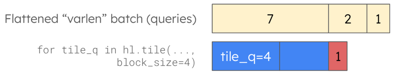
Figure 2: Accessing the flattened “varlen” tensor with fixed tile sizes requires manual masking.
So, if we would loop through this with always the same tile size (4 in this example), we would have tokens of the second request in the second tile, together with the last three of the first request! Also, the next tile would mix tokens from the second and third request. Yet, we cannot change the tile size for every sequence in a batch, since each compiled kernel can have only one tile size (remember, it is a compile time constant). One solution would have been to use only block sizes of 1 here, but as we know from our development of the Triton Attention Backend in vLLM, this performs very badly in general.
Hence, the only other option was that we adjust the index of the tile and apply manual masking using hl.load.
adjusted_tile_q_index = query_start + tile_q.begin + hl.arange(q_block_size)
query_head_offset = tile_m.begin + hl.arange(num_queries_per_kv)
q_load_mask = adjusted_tile_q_index[:, None, None] < query_end

# (tile_q, tile_m, HEAD_SIZE)
q = hl.load(t_query,
            [adjusted_tile_q_index, query_head_offset, hl.arange(head_size)],
            extra_mask=q_load_mask)
Overall, this kernel implementation in Helion requires 133 lines of code (vLLM formatting with comments) vs. 295 in Triton. Check it out here.
For us, writing the Helion kernel was very straightforward compared to writing the Triton version, despite the algorithmic changes we had to make due to Helion’s programming model. In Triton, a lot of time and effort (and lines of code) are spent to make sure all tiles have the right masks and boundaries, which requires manually taking care of tensor strides and offsets in all dimensions. Helion does this automatically and also correctly, which saves a lot of effort for the developer (esp. debugging!).
In addition, Helion handles other low-level details like actual launch grid implementation, tile size discovery, or tensor memory allocation via autotuning.
Autotuning
One of Helion’s strengths and core features is autotuning. Not only can it search across a variety of different tuning knobs, it also detects all possible valid values of these knobs by itself. The user just needs to define the lower and upper bounds of tiles or block sizes. This could also be done like:
for tile_n in hl.tile(seqlen//page_size, block_size=None):
This is in strong contrast to Triton, where a user needs to list all possible valid configurations (which is usually done with a lot of nested num_stages=s for s in [1, 2, 3, 4, 5, 6, 8, 42] …). In addition to the less-comfortable API, this also risks that a user easily misses a combination that would prove quite powerful on one platform. Helion’s approach solves this problem by requiring the user to define the shapes only on a symbolic level and then deriving all of the possible combinations.
If it is not the outer-most hl.tile loop, which will become the launch grid, the boundaries of the tiles can be derived from the tensor shapes.
Helion also checks the correctness of each kernel variant that is created during autotuning, compared to a default configuration, and discards all experiments where numerical errors are too high. In the beginning of our experiments, this baseline (or called “default configuration” by Helion) was derived automatically as somewhere “in the middle” of the discovered search space. However, this auto-discovery created some problems for us, since the result was an invalid configuration for our kernel, which would not work with the page size of 16 in vLLM. Hence, autotuning didn’t work at all and we had to patch Helion and define a default configuration manually.
Yes, Helion is still only beta and in active development and this issue was later fixed by allowing the user to define an external function as autotune baseline: autotune_baseline_fn=callable(). This feature solved our issue and we could then define our existing Triton implementation as baseline, from which we know it would give a very good performance and correct results. This greatly simplified and enhanced the autotuning process for us.
Another feature we really appreciate is the “effort level” of autotuning, which Helion added as a user-defined setting: autotune_effort=, which can be ‘none’, ‘quick’, or ‘full’. From our experience in developing the Triton attention backend in vLLM, we know that due to the paged memory and the resulting limited number of valid configurations, the autotuning process is constrained and it usually does not pay off to do days of autotuning. Hence, once this feature was available, we set the effort to quick. But as usual, terms like “quick” and “slow” are relative, and the quick mode of Helions autotuner still required 10 hours to tune our kernel for 72 different scenarios (like batch size, sequence lengths, head size, etc.). Which was faster than the 25 hours it takes with the “full” (or default) setting, but maybe not as “quick” as we would have wished.
Once the autotuner finishes, it also prints out the recommended best configuration:
[2752s] Autotuning complete in 2752.1s after searching 5353 configs.

One can hardcode the best config and skip autotuning with:

@helion.kernel(config=helion.Config(
     block_sizes=[32, 4],
     indexing=['pointer', 'pointer', 'pointer', 'pointer',
'tensor_descriptor', 'pointer', 'tensor_descriptor', 'pointer',
'tensor_descriptor'],
l2_groupings=[2],
load_eviction_policies=['', '', '', '', '', 'last', 'last', ''],
loop_orders=[[1, 2, 0], [1,0]],
num_stages=6, num_warps=8, pid_type='flat',
range_flattens=[None, True, True, True],
range_multi_buffers=[None,  None, None, False],
range_num_stages=[], range_unroll_factors=[0, 1,  2, 1],
range_warp_specializes=[]), static_shapes=False)
This gives another impression about all the different configurations knobs Helion can explore. Therefore, it is important and consequential that Helion invests a lot in different autotuning algorithms. Currently, genetic algorithms are used as the default.
In the example shown above, Helion finds the tile sizes of 32 tokens (TILE_Q) and 4 pages (TILE_N, equivalent to 64 tokens) as the best. It also figures out how to address all the tensors involved, or if loops should be flattened and reordered.
A detailed discussion of all the knobs is beyond the scope of this blog post.
Our experience with autotuning the Triton kernels taught us that it is a good trade-off to tune for a broad range of scenarios (in a microbenchmark setting) and then select only a handful of configurations to be used in vLLM and use decision trees or other heuristics to select between them.
However, one disadvantage for the current version of Helion is that it expects one configuration for the complete kernel and we cannot differentiate between configurations that would be beneficial for a prefill batch or decode batch, as we can do in Triton. Hence, for the experiments in this blog, we settled on 6 configurations to be tuned “live” at vLLM deployment in the case it runs on NVIDIA, and 7 for AMD GPUs.
Performance Evaluation
Having a good developer experience is of course nice, but we still might not use Helion if the performance would be worse than what we could do with Triton. Hence, we benchmarked our new paged attention in Helion against our established Triton kernel on NVIDIA H100 and AMD MI300X. For use cases like inference servers, we always have to look at two aspects: How the kernel performs individually and how the new kernel affects the complete system, i.e. vLLM. Therefore, we first analyze the kernel performance alone in micro-benchmarks and then, in a second step, perform an end-to-end analysis.
Micro-Benchmarks
To analyze the kernel performance, we used our microbenchmark suite, which we also used for development of the vLLM Triton attention backend. Here, we base our test parameters on the Llama3.1-8B architecture (128 head size, 32 query heads, and 8 KV heads) and vary sequence lengths and batch sizes based on real-world samples. The sequences contained within a batch have variable lengths, i.e. the “varlen” mode, as is the default in vLLM. We used Helion 0.2.4, Triton 3.5.0 and PyTorch 2.9 for all experiments.
For each GPU platform, we made two plots with the same data, but in one plot sorted by the share of decode requests within a batch, and in the other by maximum sequence length within a mixed prefill-decode varlen batch. Please note that all measurements are done with CUDA/HIP graphs enabled, so we do not evaluate any software overhead like compile time or launch time, just pure kernel performance. Since we focus on the comparison between Triton and Helion kernels, we normalized all data with the leftmost Triton result in each plot.
Each plot shows three results: The Triton 2D kernel (as it is in vLLM today) as baseline, the Helion kernel with dynamic shapes (static_shapes=False) with the selected configurations used for small-scale “live” autotuning in vLLM for each platform, and the Helion kernel with static shapes (static_shapes=True) and full autotuning. Of course, to combine dynamic shapes with full autotuning and static shapes with quick autotuning would also be valid combinations, but we don’t plot them here for clarity. Instead, we selected the both “extremes”: First, “fewer” optimizations per request, which means dynamic shapes and quick autotuning over the selected configurations. And second the scenario with the most possible optimizations, which means static shapes and full tuning for each of them.
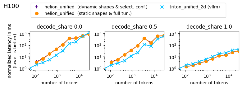
Figure 3: Microbenchmark on H100. The latencies are sorted by share of decode requests within a batch. The sequences contained within a batch have variable lengths with a median of 40% of the maximum sequence, as it could occur in real-world online inference scenarios. The combined number of tokens in a batch is denoted as x-axis.
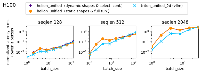
Figure 4: Microbenchmark on H100. Same setup and results as the Figure above, but here the latencies are sorted by maximum sequence length within a batch, with prefill, partial prefill, and decodes combined.
As can be seen for an H100, our Helion paged attention implementation is already outperforming the Triton 2D attention kernel for decodes, and is on-par for large batches in prefill. Our data shows that the performance of the Helion kernel ranges between 29% and 137% vs Triton for prefill requests, and between 132% and 153% for decode-only requests. Also, the plots show barely any difference between the Helion variant with static shapes and the one without. This fact is important for end-to-end measurements and will be discussed in the next Section.
The gap in the prefill can be explained by the smaller launch grid of the Helion kernel vs the Triton kernel. As discussed above, the Helion kernel parallelizes only over the query head and batch dimensions, not along the queries itself. This is in contrast to the Triton 2d kernel, where the two dimensions are the batch dimension (as in Helion) and a mix between query-head and query-tokens as second dimension. Hence, optimizing the launch grid of the Helion kernel is another optimization avenue.
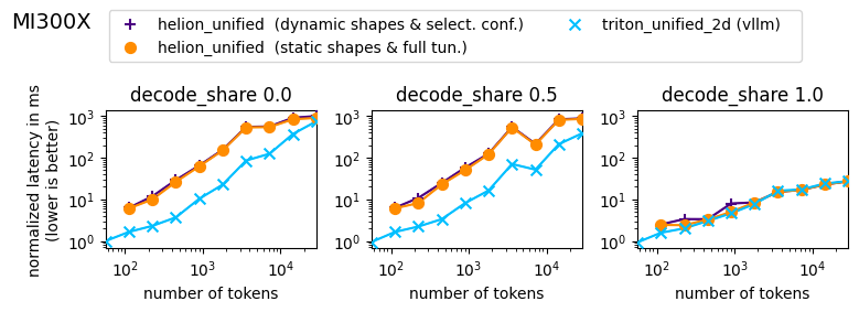
Figure 5: Microbenchmark on MI300X. The latencies are sorted by share of decode requests within a batch. The sequences contained within a batch have variable lengths with a median of 40% of the maximum sequence, as it could occur in real-world online inference scenarios. The combined number of tokens in a batch is denoted as x-axis.
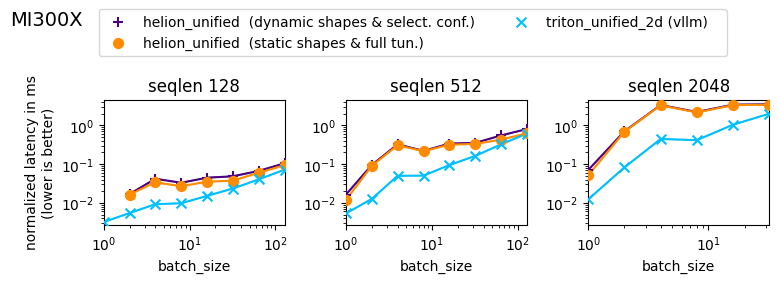
Figure 6: Microbenchmark on MI300X. Same setup and results as the Figure above, but here the latencies are sorted by maximum sequence length within a batch, with prefill, partial prefill, and decodes combined.
For MI300X, the results look a little bit different as the gap for prefills is larger. Here, the performance of the Helion kernel vs. the Triton kernel varies between 13% and 75% for prefill requests and between 58% and 107% for decode-only batches.
However, also here the Helion kernel is on-par or outperforms the Triton kernel for decode-only requests, and therefore we can consider our kernel implementation as platform and performance portable.
End-to-End in vLLM
Being a big fan of vLLM, we of course wanted to evaluate how our Helion paged attention algorithm can perform in realistic and relevant end-to-end scenarios.
Therefore, we wrote a “helion_attn” backend, similar to our Triton attention backend and evaluated its performance. We also submitted a draft PR for this.
For evaluation, we used vLLM built-in serving benchmark script with the popular ShareGPT benchmark. We also disabled prefix caching.
VLLM_ATTENTION_BACKEND=EXPERIMENTAL_HELION_ATTN vllm serve \
     meta-llama/llama3.1-8b-instruct/ \
    --disable-log-requests --no-enable-prefix-caching

vllm bench serve --model meta-llama/llama3.1-8b-instruct/ \
    --dataset-name sharegpt \
    --dataset-path ShareGPT_V3_unfiltered_cleaned_split.json \
    --ignore_eos
This setup evaluates the performance of the vLLM inference server “end-to-end”, because the performance is measured by the client, which is sending requests to the server as a real user would be. This means that the client also does not assume any knowledge of the state of the inference server, i.e. how many requests are currently running or which “shapes” the requests should have for good kernel performance. In the particular benchmark used in these experiments, the client sends 1000 requests at once and the vLLM server then has to process them as-fast-as possible, which includes scheduling very large batches and especially decode-only batches.
We compared our experimental Helion attention backend with our Triton backend as it is in vLLM today. Both backends use full CUDA/HIP graphs for mixed and decode only batches. One difference is that the Triton attention backend in vLLM today does not do “live” tuning and instead selects between four different configurations with if-else statements. This is in contrast to our proof-of-concept Helion attention backend, which uses the autotuner at runtime to choose from 6 or 7 configurations, depending on the platform. To be fair for both implementations, we always do two warmup benchmark runs to allow the autotuner to run and Helion and Triton JIT compilers to compile most of the relevant kernel versions. Each plot shows three results: The performance of the triton_attn backend as it is in vLLM today as baseline, the performance of our Helion kernel with static shapes, and the performance of our Helion kernel with dynamic shapes. Also in these experiments, we normalized the results with the Triton results.
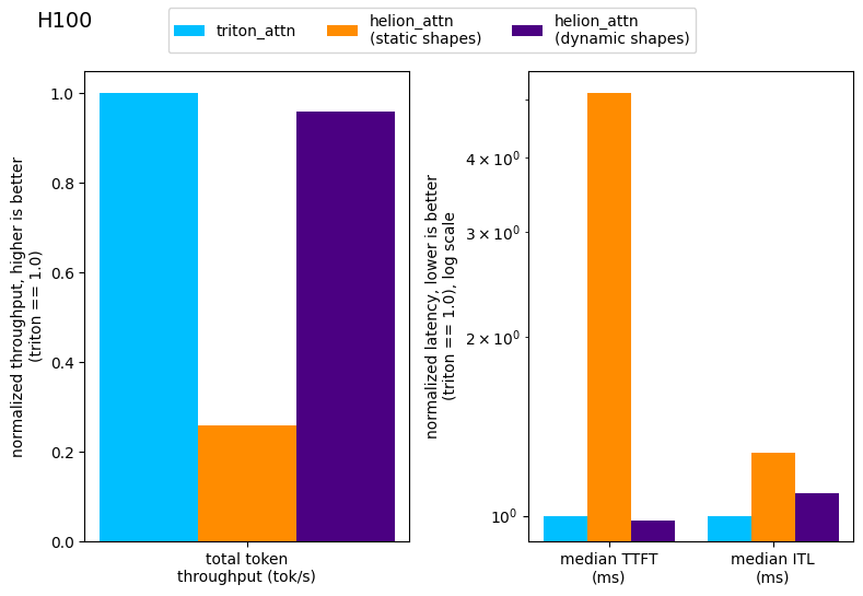
Figure 7: End-to-end performance measurements using vllm bench with Llama3.1 8B and the ShareGPT dataset on H100.
As can be seen in the Figure, Helion with static shapes achieves only roughly 26% of Triton’s total throughput, while Helion with dynamic shapes achieves 96% of the total token throughput and is also on par in TTFT (Time-to-first-token, i.e. the prefill time) and very close in ITL (Inter-token-latency, i.e. the time to decode one more token).
This experiment highlighted one important reality of inference servers: Request shapes are diverse, plentiful, and not known in advance. Furthermore, the scheduled batch shapes also depend on various other aspects like the order in which requests arrive. Hence, even if the same benchmark was run as warmup, using Helion with static shapes triggers re-compilation for nearly every request, since shapes of the query tensor are rarely exactly the same. Since this is an end-to-end experiment, these compilation times are reflected in the measured latencies and throughput. This way of evaluating the performance of our kernel implementation is different then looking at the raw kernel performance as done in micro-benchmarks, but it reflects the real-world performance that would be experienced by users of vLLM.
Consequently, Helion with static shapes performs poorly due to its huge JIT overhead that outweighs the (small) performance gains in kernel runtime. Please note, due to unrecoverable crashes of the generated Triton code during “live” autotuning, we had to disable it for the end-to-end experiments with static shapes and used the configuration with the best decode performance, as determined in micro-benchmarks. This limitation of the experiments could explain a small part of the gap in TTFT between static and dynamic shapes, but not the gap in ITL nor the big difference in throughput. Static shapes are enabled by default and allow Helion to optimize the performance using hard-coded tensor shapes in the generated Triton code. Static shapes are usually mentioned as performance optimization in Helion, but for highly dynamic usage scenarios like vLLM they are not.
More surprising are the corresponding results of the micro-benchmarks: Even if looking at the pure kernel performance, there is barely a difference between optimizing for static shapes or not. We suspect that the fact that the inputs to a paged attention kernel are actually quite shape-constrained contributes a lot to the minimal performance difference between static and dynamic shape compilation in Helion. For example, the size of the matrix multiplications always need to align with the KV cache page size (or block size) of vLLM and compile-time optimizations like loop fusion cannot change this.
One additional surprise in these end-to-end results was that the TTFT of Helion is actually on par with Triton in this specific benchmark, because here the prefill batches are larger and more uniform than in our microbenchmark setup.
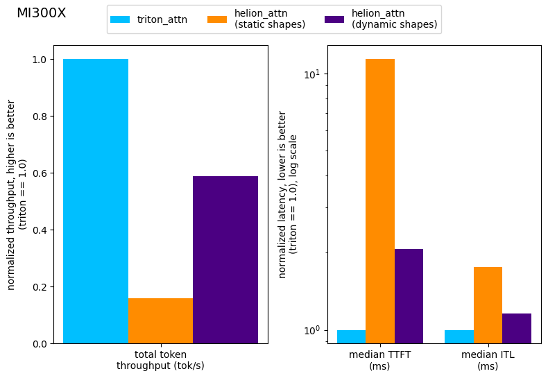
Figure 8: End-to-end performance measurements using vllm bench with Llama3.1 8B and the ShareGPT dataset on MI300X.
On MI300X, our backend works as well, but achieves only 59% of the total token throughput using dynamic shapes. This result is not surprising, because already our micro-benchmark showed that on MI300X the gap between the Helion kernel and the Triton kernel for prefills is larger.
Lessons Learned and Conclusion
We enjoyed this experiment and see Helion as both a very handy language and a powerful autotuner. Overall we spent less than three weeks on the experiments described in this blog post and are quite surprised by the impressive results.
Of course, there are many options left to further optimize this implementation of paged attention in Helion. For example, to balance long prefills, long decodes, or very large batches. This would require implementing different launch grids or parallelizations along the queries in Helion and further research to determine the optimal heuristics to choose between different kernel versions, similar to how it is implemented in our Triton attention backend. This missing fine-grained optimization also explains the gap in performance between Triton and Helion implementation in the reported experiments. In the best case, we could teach the Helion autotuner to do this balance automatically (see further discussion). Since these trade-offs are all platform dependent, we think the autotuner of Helion is well-suited to automate this reliably and fast. However, also in this context, we need to find a good balance to re-trigger Helion tuning and JIT vs. low-latency execution of the kernels that were already compiled by using heuristics to select configurations (see further discussion).
Another possible optimization for our experimental vLLM backend would be to use static shapes during CUDA/HIP graph capture, since there the additional JIT overhead does not matter and the shapes of a recorded CUDA/HIP graph are static. Hence, here it would be safe to let the compiler optimize more aggressively taking the shapes into account. However, we then have to switch to dynamic shapes afterwards during runtime.
During our experiments, we realized that for development with Helion kernels, we also need an extensive, automated, and reliable micro-benchmark suite to understand the detailed performance of the kernel in a large number of use cases. This is similar to how we learned to develop our Triton kernels, and therefore, we adapted our micro-benchmark suite that we initially built for our work with Triton.
The single most-useful “Helion command” turned out to be tensor.view, to understand early if the Helion compiler considers the shape of tensors to be the same as we expect. This made debugging compiler errors that only print out symbolic shapes a lot easier.
Finally, we would like to add some pre-trained heuristics or decision trees to Helion, to have a middle ground between hour-long autotuning and just one configuration for all cases in low-latency scenarios such as vLLM.
In conclusion, we think Helion is an exciting and quite useful addition to the PyTorch ecosystem, and we are curious how it will impact vLLM.
Acknowledgments
This work was supported by the AI platform team at IBM Research, in particular we would like to thank our colleagues: Thomas Parnell, Jan van Lunteren, Mudhakar Srivatsa, and Raghu Ganti. Also, we would like to thank Jason Ansel and the Helion team at Meta for their feedback and support, especially the fast fixing of the bugs we reported, sometimes even within 24 hours.