Ensuring the right memory format for your inputs can significantly impact the running time of your PyTorch vision models. When in doubt, choose a Channels Last memory format.
When dealing with vision models in PyTorch that accept multimedia (for example image Tensorts) as input, the Tensor’s memory format can significantly impact the inference execution speed of your model on mobile platforms when using the CPU backend along with XNNPACK. This holds true for training and inference on server platforms as well, but latency is particularly critical for mobile devices and users.
Outline of this article
- Deep Dive into matrix storage/memory representation in C++. Introduction to Row and Column major order.
- Impact of looping over a matrix in the same or different order as the storage representation, along with an example.
- Introduction to Cachegrind; a tool to inspect the cache friendliness of your code.
- Memory formats supported by PyTorch Operators.
- Best practices example to ensure efficient model execution with XNNPACK optimizations
Matrix Storage Representation in C++
Images are fed into PyTorch ML models as multi-dimensional Tensors. These Tensors have specific memory formats. To understand this concept better, let’s take a look at how a 2-d matrix may be stored in memory.
Broadly speaking, there are 2 main ways of efficiently storing multi-dimensional data in memory.
- Row Major Order: In this format, the matrix is stored in row order, with each row stored before the next row in memory. I.e. row N comes before row N+1.
- Column Major Order: In this format, the matrix is stored in column-order, with each column stored before the next column in memory. I.e. column N comes before column N+1.
You can see the differences graphically below.
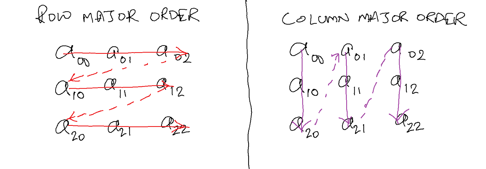
C++ stores multi-dimensional data in row-major format.
Efficiently accessing elements of a 2d matrix
Similar to the storage format, there are 2 ways to access data in a 2d matrix.
- Loop Over Rows first: All elements of a row are processed before any element of the next row.
- Loop Over Columns first: All elements of a column are processed before any element of the next column.
For maximum efficiency, one should always access data in the same format in which it is stored. I.e. if the data is stored in row-major order, then one should try to access it in that order.
The code below (main.cpp) shows 2 ways of accessing all the elements of a 2d 4000×4000 matrix.
#include <iostream>
#include <chrono>

// loop1 accesses data in matrix 'a' in row major order,
// since i is the outer loop variable, and j is the
// inner loop variable.
int loop1(int a[4000][4000]) {
 int s = 0;
 for (int i = 0; i < 4000; ++i) {
   for (int j = 0; j < 4000; ++j) {
     s += a[i][j];
   }
 }
 return s;
}

// loop2 accesses data in matrix 'a' in column major order
// since j is the outer loop variable, and i is the
// inner loop variable.
int loop2(int a[4000][4000]) {
 int s = 0;
 for (int j = 0; j < 4000; ++j) {
   for (int i = 0; i < 4000; ++i) {
     s += a[i][j];
   }
 }
 return s;
}

int main() {
 static int a[4000][4000] = {0};
 for (int i = 0; i < 100; ++i) {
   int x = rand() % 4000;
   int y = rand() % 4000;
   a[x][y] = rand() % 1000;
 }

 auto start = std::chrono::high_resolution_clock::now();
 auto end = start;
 int s = 0;

#if defined RUN_LOOP1
 start = std::chrono::high_resolution_clock::now();

 s = 0;
 for (int i = 0; i < 10; ++i) {
   s += loop1(a);
   s = s % 100;
 }
 end = std::chrono::high_resolution_clock::now();

 std::cout << "s = " << s << std::endl;
 std::cout << "Time for loop1: "
   << std::chrono::duration<double, std::milli>(end - start).count()
   << "ms" << std::endl;
#endif

#if defined RUN_LOOP2
 start = std::chrono::high_resolution_clock::now();
 s = 0;
 for (int i = 0; i < 10; ++i) {
   s += loop2(a);
   s = s % 100;
 }
 end = std::chrono::high_resolution_clock::now();

 std::cout << "s = " << s << std::endl;
 std::cout << "Time for loop2: "
   << std::chrono::duration<double, std::milli>(end - start).count()
   << "ms" << std::endl;
#endif
}


Let’s build and run this program and see what it prints.

g++ -O2 main.cpp -DRUN_LOOP1 -DRUN_LOOP2
./a.out


Prints the following:

s = 70
Time for loop1: 77.0687ms
s = 70
Time for loop2: 1219.49ms
loop1() is 15x faster than loop2(). Why is that? Let’s find out below!
Measure cache misses using Cachegrind
Cachegrind is a cache profiling tool used to see how many I1 (first level instruction), D1 (first level data), and LL (last level) cache misses your program caused.
Let’s build our program with just loop1() and just loop2() to see how cache friendly each of these functions is.
Build and run/profile just loop1()
g++ -O2 main.cpp -DRUN_LOOP1
valgrind --tool=cachegrind ./a.out
Prints:
==3299700==
==3299700== I   refs:      643,156,721
==3299700== I1  misses:          2,077
==3299700== LLi misses:          2,021
==3299700== I1  miss rate:        0.00%
==3299700== LLi miss rate:        0.00%
==3299700==
==3299700== D   refs:      160,952,192  (160,695,444 rd   + 256,748 wr)
==3299700== D1  misses:     10,021,300  ( 10,018,723 rd   +   2,577 wr)
==3299700== LLd misses:     10,010,916  ( 10,009,147 rd   +   1,769 wr)
==3299700== D1  miss rate:         6.2% (        6.2%     +     1.0%  )
==3299700== LLd miss rate:         6.2% (        6.2%     +     0.7%  )
==3299700==
==3299700== LL refs:        10,023,377  ( 10,020,800 rd   +   2,577 wr)
==3299700== LL misses:      10,012,937  ( 10,011,168 rd   +   1,769 wr)
==3299700== LL miss rate:          1.2% (        1.2%     +     0.7%  )
Build and run/profile just loop2()
g++ -O2 main.cpp -DRUN_LOOP2
valgrind --tool=cachegrind ./a.out
Prints:
==3300389==
==3300389== I   refs:      643,156,726
==3300389== I1  misses:          2,075
==3300389== LLi misses:          2,018
==3300389== I1  miss rate:        0.00%
==3300389== LLi miss rate:        0.00%
==3300389==
==3300389== D   refs:      160,952,196  (160,695,447 rd   + 256,749 wr)
==3300389== D1  misses:    160,021,290  (160,018,713 rd   +   2,577 wr)
==3300389== LLd misses:     10,014,907  ( 10,013,138 rd   +   1,769 wr)
==3300389== D1  miss rate:        99.4% (       99.6%     +     1.0%  )
==3300389== LLd miss rate:         6.2% (        6.2%     +     0.7%  )
==3300389==
==3300389== LL refs:       160,023,365  (160,020,788 rd   +   2,577 wr)
==3300389== LL misses:      10,016,925  ( 10,015,156 rd   +   1,769 wr)
==3300389== LL miss rate:          1.2% (        1.2%     +     0.7%  )
The main differences between the 2 runs are:
- D1 misses: 10M v/s 160M
- D1 miss rate: 6.2% v/s 99.4%
As you can see, loop2() causes many many more (~16x more) L1 data cache misses than loop1(). This is why loop1() is ~15x faster than loop2().
Memory Formats supported by PyTorch Operators
While PyTorch operators expect all tensors to be in Channels First (NCHW) dimension format, PyTorch operators support 3 output memory formats.
- Contiguous: Tensor memory is in the same order as the tensor’s dimensions.
- ChannelsLast: Irrespective of the dimension order, the 2d (image) tensor is laid out as an HWC or NHWC (N: batch, H: height, W: width, C: channels) tensor in memory. The dimensions could be permuted in any order.
- ChannelsLast3d: For 3d tensors (video tensors), the memory is laid out in THWC (Time, Height, Width, Channels) or NTHWC (N: batch, T: time, H: height, W: width, C: channels) format. The dimensions could be permuted in any order.
The reason that ChannelsLast is preferred for vision models is because XNNPACK (kernel acceleration library) used by PyTorch expects all inputs to be in Channels Last format, so if the input to the model isn’t channels last, then it must first be converted to channels last, which is an additional operation.
Additionally, most PyTorch operators preserve the input tensor’s memory format, so if the input is Channels First, then the operator needs to first convert to Channels Last, then perform the operation, and then convert back to Channels First.
When you combine it with the fact that accelerated operators work better with a channels last memory format, you’ll notice that having the operator return back a channels-last memory format is better for subsequent operator calls or you’ll end up having every operator convert to channels-last (should it be more efficient for that specific operator).
From the XNNPACK home page:
“All operators in XNNPACK support NHWC layout, but additionally allow custom stride along the Channel dimension”.
PyTorch Best Practice
The best way to get the most performance from your PyTorch vision models is to ensure that your input tensor is in a Channels Last memory format before it is fed into the model.
You can get even more speedups by optimizing your model to use the XNNPACK backend (by simply calling optimize_for_mobile() on your torchscripted model). Note that XNNPACK models will run slower if the inputs are contiguous, so definitely make sure it is in Channels-Last format.
Working example showing speedup
Run this example on Google Colab – note that runtimes on colab CPUs might not reflect accurate performance; it is recommended to run this code on your local machine.
import torch
from torch.utils.mobile_optimizer import optimize_for_mobile
import torch.backends.xnnpack
import time

print("XNNPACK is enabled: ", torch.backends.xnnpack.enabled, "\n")

N, C, H, W = 1, 3, 200, 200
x = torch.rand(N, C, H, W)
print("Contiguous shape: ", x.shape)
print("Contiguous stride: ", x.stride())
print()

xcl = x.to(memory_format=torch.channels_last)
print("Channels-Last shape: ", xcl.shape)
print("Channels-Last stride: ", xcl.stride())

## Outputs:

# XNNPACK is enabled:  True

# Contiguous shape:  torch.Size([1, 3, 200, 200])
# Contiguous stride:  (120000, 40000, 200, 1)

# Channels-Last shape:  torch.Size([1, 3, 200, 200])
# Channels-Last stride:  (120000, 1, 600, 3)
The input shape stays the same for contiguous and channels-last formats. Internally however, the tensor’s layout has changed as you can see in the strides. Now, the number of jumps required to go across channels is only 1 (instead of 40000 in the contiguous tensor). This better data locality means convolution layers can access all the channels for a given pixel much faster. Let’s see now how the memory format affects runtime:
from torchvision.models import resnet34, resnet50, resnet101

m = resnet34(pretrained=False)
# m = resnet50(pretrained=False)
# m = resnet101(pretrained=False)

def get_optimized_model(mm):
  mm = mm.eval()
  scripted = torch.jit.script(mm)
  optimized = optimize_for_mobile(scripted)  # explicitly call the xnnpack rewrite
  return scripted, optimized


def compare_contiguous_CL(mm):
  # inference on contiguous
  start = time.perf_counter()
  for i in range(20):
    mm(x)
  end = time.perf_counter()
  print("Contiguous: ", end-start)

  # inference on channels-last
  start = time.perf_counter()
  for i in range(20):
    mm(xcl)
  end = time.perf_counter()
  print("Channels-Last: ", end-start)

with torch.inference_mode():
  scripted, optimized = get_optimized_model(m)

  print("Runtimes for torchscripted model: ")
  compare_contiguous_CL(scripted.eval())
  print()
  print("Runtimes for mobile-optimized model: ")
  compare_contiguous_CL(optimized.eval())


## Outputs (on an Intel Core i9 CPU):

# Runtimes for torchscripted model:
# Contiguous:  1.6711160129999598
# Channels-Last:  1.6678222839999535

# Runtimes for mobile-optimized model:
# Contiguous:  0.5712863490000473
# Channels-Last:  0.46113000699995155
Conclusion
The Memory Layout of an input tensor can significantly impact a model’s running time. For Vision Models, prefer a Channels Last memory format to get the most out of your PyTorch models.