Quantization is a cheap and easy way to make your DNN run faster and with lower memory requirements. PyTorch offers a few different approaches to quantize your model. In this blog post, we’ll lay a (quick) foundation of quantization in deep learning, and then take a look at how each technique looks like in practice. Finally we’ll end with recommendations from the literature for using quantization in your workflows.

Fig 1. PyTorch <3 Quantization
Contents
- Fundamentals of Quantization
- In PyTorch
- Sensitivity Analysis
- Recommendations for your workflow
- References
Fundamentals of Quantization
If someone asks you what time it is, you don’t respond “10:14:34:430705”, but you might say “a quarter past 10”.
Quantization has roots in information compression; in deep networks it refers to reducing the numerical precision of its weights and/or activations.
Overparameterized DNNs have more degrees of freedom and this makes them good candidates for information compression [1]. When you quantize a model, two things generally happen – the model gets smaller and runs with better efficiency. Hardware vendors explicitly allow for faster processing of 8-bit data (than 32-bit data) resulting in higher throughput. A smaller model has lower memory footprint and power consumption [2], crucial for deployment at the edge.
Mapping function
The mapping function is what you might guess – a function that maps values from floating-point to integer space. A commonly used mapping function is a linear transformation given by , where
is the input and
are quantization parameters.
To reconvert to floating point space, the inverse function is given by .
, and their difference constitutes the quantization error.
Quantization Parameters
The mapping function is parameterized by the scaling factor and zero-point
.
is simply the ratio of the input range to the output range
where [] is the clipping range of the input, i.e. the boundaries of permissible inputs. [
] is the range in quantized output space that it is mapped to. For 8-bit quantization, the output range
.
acts as a bias to ensure that a 0 in the input space maps perfectly to a 0 in the quantized space.
Calibration
The process of choosing the input clipping range is known as calibration. The simplest technique (also the default in PyTorch) is to record the running mininmum and maximum values and assign them to and
. TensorRT also uses entropy minimization (KL divergence), mean-square-error minimization, or percentiles of the input range.
In PyTorch, Observer modules (code) collect statistics on the input values and calculate the qparams . Different calibration schemes result in different quantized outputs, and it’s best to empirically verify which scheme works best for your application and architecture (more on that later).
from torch.quantization.observer import MinMaxObserver, MovingAverageMinMaxObserver, HistogramObserver
C, L = 3, 4
normal = torch.distributions.normal.Normal(0,1)
inputs = [normal.sample((C, L)), normal.sample((C, L))]
print(inputs)

# >>>>>
# [tensor([[-0.0590,  1.1674,  0.7119, -1.1270],
#          [-1.3974,  0.5077, -0.5601,  0.0683],
#          [-0.0929,  0.9473,  0.7159, -0.4574]]]),

# tensor([[-0.0236, -0.7599,  1.0290,  0.8914],
#          [-1.1727, -1.2556, -0.2271,  0.9568],
#          [-0.2500,  1.4579,  1.4707,  0.4043]])]

observers = [MinMaxObserver(), MovingAverageMinMaxObserver(), HistogramObserver()]
for obs in observers:
  for x in inputs: obs(x)
  print(obs.__class__.__name__, obs.calculate_qparams())

# >>>>>
# MinMaxObserver (tensor([0.0112]), tensor([124], dtype=torch.int32))
# MovingAverageMinMaxObserver (tensor([0.0101]), tensor([139], dtype=torch.int32))
# HistogramObserver (tensor([0.0100]), tensor([106], dtype=torch.int32))
Affine and Symmetric Quantization Schemes
Affine or asymmetric quantization schemes assign the input range to the min and max observed values. Affine schemes generally offer tighter clipping ranges and are useful for quantizing non-negative activations (you don’t need the input range to contain negative values if your input tensors are never negative). The range is calculated as . Affine quantization leads to more computationally expensive inference when used for weight tensors [3].
Symmetric quantization schemes center the input range around 0, eliminating the need to calculate a zero-point offset. The range is calculated as . For skewed signals (like non-negative activations) this can result in bad quantization resolution because the clipping range includes values that never show up in the input (see the pyplot below).
act =  torch.distributions.pareto.Pareto(1, 10).sample((1,1024))
weights = torch.distributions.normal.Normal(0, 0.12).sample((3, 64, 7, 7)).flatten()

def get_symmetric_range(x):
  beta = torch.max(x.max(), x.min().abs())
  return -beta.item(), beta.item()

def get_affine_range(x):
  return x.min().item(), x.max().item()

def plot(plt, data, scheme):
  boundaries = get_affine_range(data) if scheme == 'affine' else get_symmetric_range(data)
  a, _, _ = plt.hist(data, density=True, bins=100)
  ymin, ymax = np.quantile(a[a>0], [0.25, 0.95])
  plt.vlines(x=boundaries, ls='--', colors='purple', ymin=ymin, ymax=ymax)

fig, axs = plt.subplots(2,2)
plot(axs[0, 0], act, 'affine')
axs[0, 0].set_title("Activation, Affine-Quantized")

plot(axs[0, 1], act, 'symmetric')
axs[0, 1].set_title("Activation, Symmetric-Quantized")

plot(axs[1, 0], weights, 'affine')
axs[1, 0].set_title("Weights, Affine-Quantized")

plot(axs[1, 1], weights, 'symmetric')
axs[1, 1].set_title("Weights, Symmetric-Quantized")
plt.show()
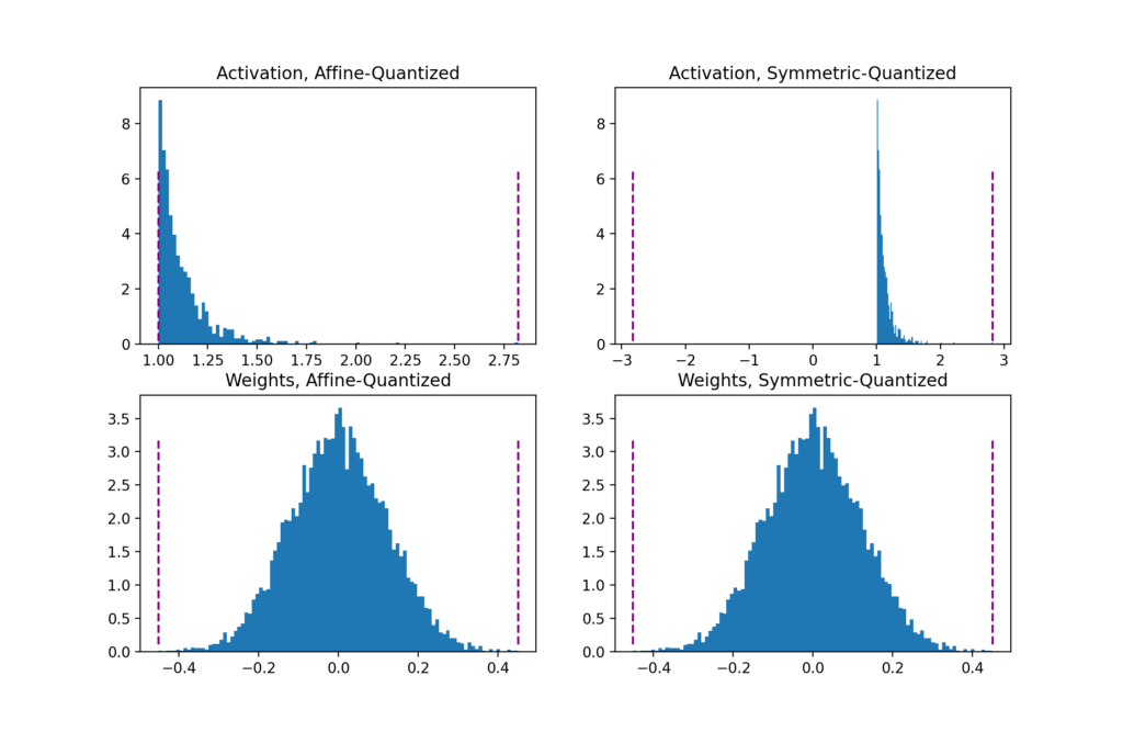
Fig 2. Clipping ranges (in purple) for affine and symmetric schemes
In PyTorch, you can specify affine or symmetric schemes while initializing the Observer. Note that not all observers support both schemes.
for qscheme in [torch.per_tensor_affine, torch.per_tensor_symmetric]:
  obs = MovingAverageMinMaxObserver(qscheme=qscheme)
  for x in inputs: obs(x)
  print(f"Qscheme: {qscheme} | {obs.calculate_qparams()}")

# >>>>>
# Qscheme: torch.per_tensor_affine | (tensor([0.0101]), tensor([139], dtype=torch.int32))
# Qscheme: torch.per_tensor_symmetric | (tensor([0.0109]), tensor([128]))
Per-Tensor and Per-Channel Quantization Schemes
Quantization parameters can be calculated for the layer’s entire weight tensor as a whole, or separately for each channel. In per-tensor, the same clipping range is applied to all the channels in a layer

Fig 3. Per-Channel uses one set of qparams for each channel. Per-tensor uses the same qparams for the entire tensor.
For weights quantization, symmetric-per-channel quantization provides better accuracies; per-tensor quantization performs poorly, possibly due to high variance in conv weights across channels from batchnorm folding [3].
from torch.quantization.observer import MovingAveragePerChannelMinMaxObserver
obs = MovingAveragePerChannelMinMaxObserver(ch_axis=0)  # calculate qparams for all `C` channels separately
for x in inputs: obs(x)
print(obs.calculate_qparams())

# >>>>>
# (tensor([0.0090, 0.0075, 0.0055]), tensor([125, 187,  82], dtype=torch.int32))
Backend Engine
Currently, quantized operators run on x86 machines via the FBGEMM backend, or use QNNPACK primitives on ARM machines. Backend support for server GPUs (via TensorRT and cuDNN) is coming soon. Learn more about extending quantization to custom backends: RFC-0019.
backend = 'fbgemm' if x86 else 'qnnpack'
qconfig = torch.quantization.get_default_qconfig(backend)
torch.backends.quantized.engine = backend
QConfig
The QConfig (code) NamedTuple stores the Observers and the quantization schemes used to quantize activations and weights.
Be sure to pass the Observer class (not the instance), or a callable that can return Observer instances. Use with_args() to override the default arguments.
my_qconfig = torch.quantization.QConfig(
  activation=MovingAverageMinMaxObserver.with_args(qscheme=torch.per_tensor_affine),
  weight=MovingAveragePerChannelMinMaxObserver.with_args(qscheme=torch.qint8)
)
# >>>>>
# QConfig(activation=functools.partial(<class 'torch.ao.quantization.observer.MovingAverageMinMaxObserver'>, qscheme=torch.per_tensor_affine){}, weight=functools.partial(<class 'torch.ao.quantization.observer.MovingAveragePerChannelMinMaxObserver'>, qscheme=torch.qint8){})
In PyTorch
PyTorch allows you a few different ways to quantize your model depending on
- if you prefer a flexible but manual, or a restricted automagic process (Eager Mode v/s FX Graph Mode)
- if qparams for quantizing activations (layer outputs) are precomputed for all inputs, or calculated afresh with each input (static v/s dynamic),
- if qparams are computed with or without retraining (quantization-aware training v/s post-training quantization)
FX Graph Mode automatically fuses eligible modules, inserts Quant/DeQuant stubs, calibrates the model and returns a quantized module – all in two method calls – but only for networks that are symbolic traceable. The examples below contain the calls using Eager Mode and FX Graph Mode for comparison.
In DNNs, eligible candidates for quantization are the FP32 weights (layer parameters) and activations (layer outputs). Quantizing weights reduces the model size. Quantized activations typically result in faster inference.
As an example, the 50-layer ResNet network has ~26 million weight parameters and computes ~16 million activations in the forward pass.
Post-Training Dynamic/Weight-only Quantization
Here the model’s weights are pre-quantized; the activations are quantized on-the-fly (“dynamic”) during inference. The simplest of all approaches, it has a one line API call in torch.quantization.quantize_dynamic. Currently only Linear and Recurrent (LSTM, GRU, RNN) layers are supported for dynamic quantization.
(+) Can result in higher accuracies since the clipping range is exactly calibrated for each input [1].
(+) Dynamic quantization is preferred for models like LSTMs and Transformers where writing/retrieving the model’s weights from memory dominate bandwidths [4].
(-) Calibrating and quantizing the activations at each layer during runtime can add to the compute overhead.
import torch
from torch import nn

# toy model
m = nn.Sequential(
  nn.Conv2d(2, 64, (8,)),
  nn.ReLU(),
  nn.Linear(16,10),
  nn.LSTM(10, 10))

m.eval()

## EAGER MODE
from torch.quantization import quantize_dynamic
model_quantized = quantize_dynamic(
    model=m, qconfig_spec={nn.LSTM, nn.Linear}, dtype=torch.qint8, inplace=False
)

## FX MODE
from torch.quantization import quantize_fx
qconfig_dict = {"": torch.quantization.default_dynamic_qconfig}  # An empty key denotes the default applied to all modules
model_prepared = quantize_fx.prepare_fx(m, qconfig_dict)
model_quantized = quantize_fx.convert_fx(model_prepared)
Post-Training Static Quantization (PTQ)
PTQ also pre-quantizes model weights but instead of calibrating activations on-the-fly, the clipping range is pre-calibrated and fixed (“static”) using validation data. Activations stay in quantized precision between operations during inference. About 100 mini-batches of representative data are sufficient to calibrate the observers [2]. The examples below use random data in calibration for convenience – using that in your application will result in bad qparams.

Fig 4. Steps in Post-Training Static Quantization
Module fusion combines multiple sequential modules (eg: [Conv2d, BatchNorm, ReLU]) into one. Fusing modules means the compiler needs to only run one kernel instead of many; this speeds things up and improves accuracy by reducing quantization error.
(+) Static quantization has faster inference than dynamic quantization because it eliminates the float<->int conversion costs between layers.
(-) Static quantized models may need regular re-calibration to stay robust against distribution-drift.
# Static quantization of a model consists of the following steps:

#     Fuse modules
#     Insert Quant/DeQuant Stubs
#     Prepare the fused module (insert observers before and after layers)
#     Calibrate the prepared module (pass it representative data)
#     Convert the calibrated module (replace with quantized version)

import torch
from torch import nn
import copy

backend = "fbgemm"  # running on a x86 CPU. Use "qnnpack" if running on ARM.

model = nn.Sequential(
     nn.Conv2d(2,64,3),
     nn.ReLU(),
     nn.Conv2d(64, 128, 3),
     nn.ReLU()
)

## EAGER MODE
m = copy.deepcopy(model)
m.eval()
"""Fuse
- Inplace fusion replaces the first module in the sequence with the fused module, and the rest with identity modules
"""
torch.quantization.fuse_modules(m, ['0','1'], inplace=True) # fuse first Conv-ReLU pair
torch.quantization.fuse_modules(m, ['2','3'], inplace=True) # fuse second Conv-ReLU pair

"""Insert stubs"""
m = nn.Sequential(torch.quantization.QuantStub(),
                  *m,
                  torch.quantization.DeQuantStub())

"""Prepare"""
m.qconfig = torch.quantization.get_default_qconfig(backend)
torch.quantization.prepare(m, inplace=True)

"""Calibrate
- This example uses random data for convenience. Use representative (validation) data instead.
"""
with torch.inference_mode():
  for _ in range(10):
    x = torch.rand(1,2, 28, 28)
    m(x)

"""Convert"""
torch.quantization.convert(m, inplace=True)

"""Check"""
print(m[[1]].weight().element_size()) # 1 byte instead of 4 bytes for FP32


## FX GRAPH
from torch.quantization import quantize_fx
m = copy.deepcopy(model)
m.eval()
qconfig_dict = {"": torch.quantization.get_default_qconfig(backend)}
# Prepare
model_prepared = quantize_fx.prepare_fx(m, qconfig_dict)
# Calibrate - Use representative (validation) data.
with torch.inference_mode():
  for _ in range(10):
    x = torch.rand(1,2,28, 28)
    model_prepared(x)
# quantize
model_quantized = quantize_fx.convert_fx(model_prepared)
Quantization-aware Training (QAT)

Fig 5. Steps in Quantization-Aware Training
The PTQ approach is great for large models, but accuracy suffers in smaller models [[6]]. This is of course due to the loss in numerical precision when adapting a model from FP32 to the INT8 realm (Figure 6(a)). QAT tackles this by including this quantization error in the training loss, thereby training an INT8-first model.
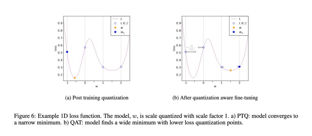
Fig 6. Comparison of PTQ and QAT convergence [3]
All weights and biases are stored in FP32, and backpropagation happens as usual. However in the forward pass, quantization is internally simulated via FakeQuantize modules. They are called fake because they quantize and immediately dequantize the data, adding quantization noise similar to what might be encountered during quantized inference. The final loss thus accounts for any expected quantization errors. Optimizing on this allows the model to identify a wider region in the loss function (Figure 6(b)), and identify FP32 parameters such that quantizing them to INT8 does not significantly affect accuracy.
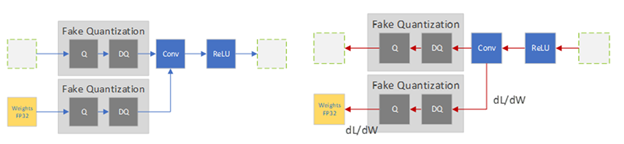
Fig 7. Fake Quantization in the forward and backward pass
Image source: https://developer.nvidia.com/blog/achieving-fp32-accuracy-for-int8-inference-using-quantization-aware-training-with-tensorrt
(+) QAT yields higher accuracies than PTQ.
(+) Qparams can be learned during model training for more fine-grained accuracy (see LearnableFakeQuantize)
(-) Computational cost of retraining a model in QAT can be several hundred epochs [1]
# QAT follows the same steps as PTQ, with the exception of the training loop before you actually convert the model to its quantized version

import torch
from torch import nn

backend = "fbgemm"  # running on a x86 CPU. Use "qnnpack" if running on ARM.

m = nn.Sequential(
     nn.Conv2d(2,64,8),
     nn.ReLU(),
     nn.Conv2d(64, 128, 8),
     nn.ReLU()
)

"""Fuse"""
torch.quantization.fuse_modules(m, ['0','1'], inplace=True) # fuse first Conv-ReLU pair
torch.quantization.fuse_modules(m, ['2','3'], inplace=True) # fuse second Conv-ReLU pair

"""Insert stubs"""
m = nn.Sequential(torch.quantization.QuantStub(),
                  *m,
                  torch.quantization.DeQuantStub())

"""Prepare"""
m.train()
m.qconfig = torch.quantization.get_default_qconfig(backend)
torch.quantization.prepare_qat(m, inplace=True)

"""Training Loop"""
n_epochs = 10
opt = torch.optim.SGD(m.parameters(), lr=0.1)
loss_fn = lambda out, tgt: torch.pow(tgt-out, 2).mean()
for epoch in range(n_epochs):
  x = torch.rand(10,2,24,24)
  out = m(x)
  loss = loss_fn(out, torch.rand_like(out))
  opt.zero_grad()
  loss.backward()
  opt.step()

"""Convert"""
m.eval()
torch.quantization.convert(m, inplace=True)
Sensitivity Analysis
Not all layers respond to quantization equally, some are more sensitive to precision drops than others. Identifying the optimal combination of layers that minimizes accuracy drop is time-consuming, so [3] suggest a one-at-a-time sensitivity analysis to identify which layers are most sensitive, and retaining FP32 precision on those. In their experiments, skipping just 2 conv layers (out of a total 28 in MobileNet v1) give them near-FP32 accuracy. Using FX Graph Mode, we can create custom qconfigs to do this easily:
# ONE-AT-A-TIME SENSITIVITY ANALYSIS

for quantized_layer, _ in model.named_modules():
  print("Only quantizing layer: ", quantized_layer)

  # The module_name key allows module-specific qconfigs.
  qconfig_dict = {"": None,
  "module_name":[(quantized_layer, torch.quantization.get_default_qconfig(backend))]}

  model_prepared = quantize_fx.prepare_fx(model, qconfig_dict)
  # calibrate
  model_quantized = quantize_fx.convert_fx(model_prepared)
  # evaluate(model)
Another approach is to compare statistics of the FP32 and INT8 layers; commonly used metrics for these are SQNR (Signal to Quantized Noise Ratio) and Mean-Squre-Error. Such a comparative analysis may also help in guiding further optimizations.
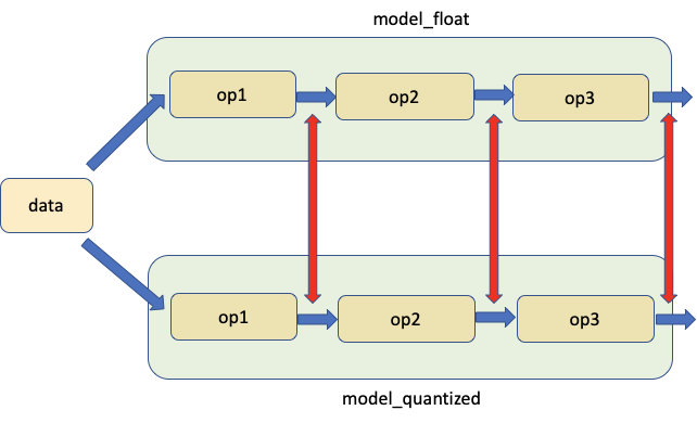
Fig 8. Comparing model weights and activations
PyTorch provides tools to help with this analysis under the Numeric Suite. Learn more about using Numeric Suite from the full tutorial.
# extract from https://pytorch.org/tutorials/prototype/numeric_suite_tutorial.html
import torch.quantization._numeric_suite as ns

def SQNR(x, y):
    # Higher is better
    Ps = torch.norm(x)
    Pn = torch.norm(x-y)
    return 20*torch.log10(Ps/Pn)

wt_compare_dict = ns.compare_weights(fp32_model.state_dict(), int8_model.state_dict())
for key in wt_compare_dict:
    print(key, compute_error(wt_compare_dict[key]['float'], wt_compare_dict[key]['quantized'].dequantize()))

act_compare_dict = ns.compare_model_outputs(fp32_model, int8_model, input_data)
for key in act_compare_dict:
    print(key, compute_error(act_compare_dict[key]['float'][0], act_compare_dict[key]['quantized'][0].dequantize()))
Recommendations for your workflow
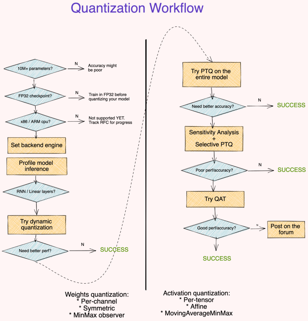
Fig 9. Suggested quantization workflow
Points to note
- Large (10M+ parameters) models are more robust to quantization error. [2]
- Quantizing a model from a FP32 checkpoint provides better accuracy than training an INT8 model from scratch.[2]
- Profiling the model runtime is optional but it can help identify layers that bottleneck inference.
- Dynamic Quantization is an easy first step, especially if your model has many Linear or Recurrent layers.
- Use symmetric-per-channel quantization with
MinMaxobservers for quantizing weights. Use affine-per-tensor quantization withMovingAverageMinMaxobservers for quantizing activations[2, 3] - Use metrics like SQNR to identify which layers are most suscpetible to quantization error. Turn off quantization on these layers.
- Use QAT to fine-tune for around 10% of the original training schedule with an annealing learning rate schedule starting at 1% of the initial training learning rate. [3]
- If the above workflow didn’t work for you, we want to know more. Post a thread with details of your code (model architecture, accuracy metric, techniques tried). Feel free to cc me @suraj.pt.
That was a lot to digest, congratulations for sticking with it! Next, we’ll take a look at quantizing a “real-world” model that uses dynamic control structures (if-else, loops). These elements disallow symbolic tracing a model, which makes it a bit tricky to directly quantize the model out of the box. In the next post of this series, we’ll get our hands dirty on a model that is chock full of loops and if-else blocks, and even uses third-party libraries in the forward call.
We’ll also cover a cool new feature in PyTorch Quantization called Define-by-Run, that tries to ease this constraint by needing only subsets of the model’s computational graph to be free of dynamic flow. Check out the Define-by-Run poster at PTDD’21 for a preview.
References
[1] Gholami, A., Kim, S., Dong, Z., Yao, Z., Mahoney, M. W., & Keutzer, K. (2021). A survey of quantization methods for efficient neural network inference. arXiv preprint arXiv:2103.13630.
[2] Krishnamoorthi, R. (2018). Quantizing deep convolutional networks for efficient inference: A whitepaper. arXiv preprint arXiv:1806.08342.
[3] Wu, H., Judd, P., Zhang, X., Isaev, M., & Micikevicius, P. (2020). Integer quantization for deep learning inference: Principles and empirical evaluation. arXiv preprint arXiv:2004.09602.
[4] PyTorch Quantization Docs