Do you use stochastic gradient descent (SGD) or Adam? Regardless of the procedure you use to train your neural network, you can likely achieve significantly better generalization at virtually no additional cost with a simple new technique now natively supported in PyTorch 1.6, Stochastic Weight Averaging (SWA) [1]. Even if you have already trained your model, it’s easy to realize the benefits of SWA by running SWA for a small number of epochs starting with a pre-trained model. Again and again, researchers are discovering that SWA improves the performance of well-tuned models in a wide array of practical applications with little cost or effort!
SWA has a wide range of applications and features:
- SWA significantly improves performance compared to standard training techniques in computer vision (e.g., VGG, ResNets, Wide ResNets and DenseNets on ImageNet and CIFAR benchmarks [1, 2]).
- SWA provides state-of-the-art performance on key benchmarks in semi-supervised learning and domain adaptation [2].
- SWA was shown to improve performance in language modeling (e.g., AWD-LSTM on WikiText-2 [4]) and policy-gradient methods in deep reinforcement learning [3].
- SWAG, an extension of SWA, can approximate Bayesian model averaging in Bayesian deep learning and achieves state-of-the-art uncertainty calibration results in various settings. Moreover, its recent generalization MultiSWAG provides significant additional performance gains and mitigates double-descent [4, 10]. Another approach, Subspace Inference, approximates the Bayesian posterior in a small subspace of the parameter space around the SWA solution [5].
- SWA for low precision training, SWALP, can match the performance of full-precision SGD training, even with all numbers quantized down to 8 bits, including gradient accumulators [6].
- SWA in parallel, SWAP, was shown to greatly speed up the training of neural networks by using large batch sizes and, in particular, set a record by training a neural network to 94% accuracy on CIFAR-10 in 27 seconds [11].
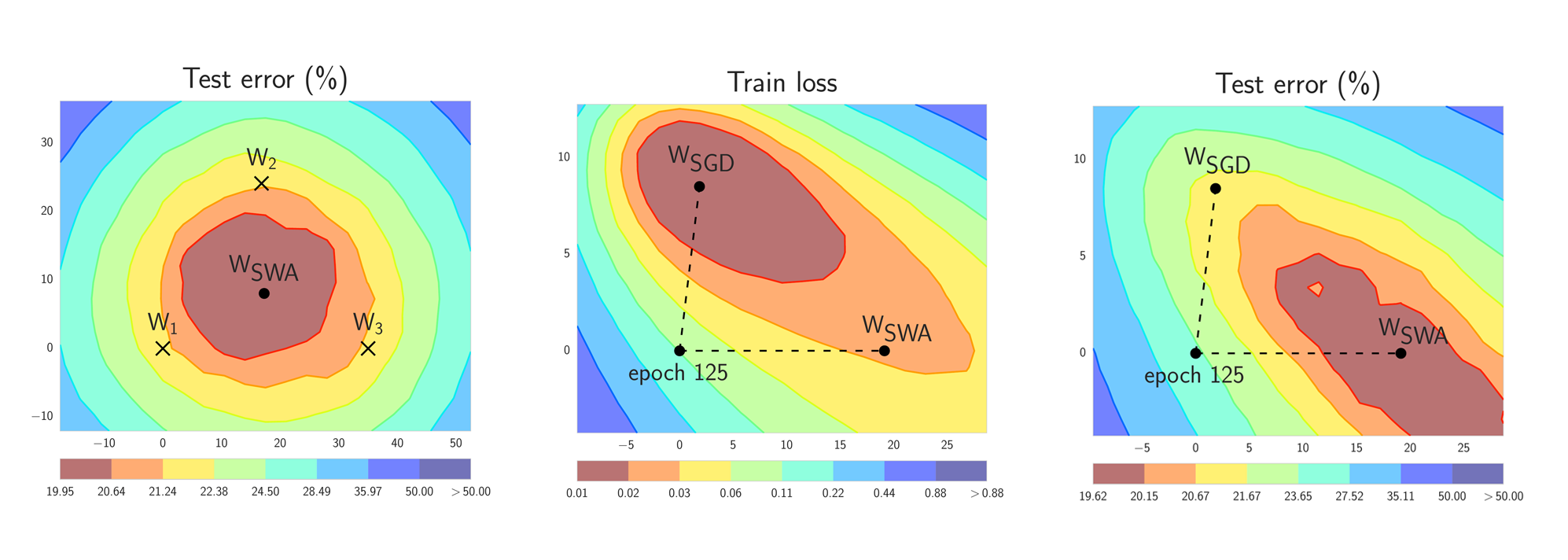
Figure 1. Illustrations of SWA and SGD with a Preactivation ResNet-164 on CIFAR-100 [1]. Left: test error surface for three FGE samples and the corresponding SWA solution (averaging in weight space). Middle and Right: test error and train loss surfaces showing the weights proposed by SGD (at convergence) and SWA, starting from the same initialization of SGD after 125 training epochs. Please see [1] for details on how these figures were constructed.
In short, SWA performs an equal average of the weights traversed by SGD (or any stochastic optimizer) with a modified learning rate schedule (see the left panel of Figure 1.). SWA solutions end up in the center of a wide flat region of loss, while SGD tends to converge to the boundary of the low-loss region, making it susceptible to the shift between train and test error surfaces (see the middle and right panels of Figure 1). We emphasize that SWA can be used with any optimizer, such as Adam, and is not specific to SGD.
Previously, SWA was in PyTorch contrib. In PyTorch 1.6, we provide a new convenient implementation of SWA in torch.optim.swa_utils.
Is this just Averaged SGD?
At a high level, averaging SGD iterates dates back several decades in convex optimization [7, 8], where it is sometimes referred to as Polyak-Ruppert averaging, or averaged SGD. But the details matter. Averaged SGD is often used in conjunction with a decaying learning rate, and an exponential moving average (EMA), typically for convex optimization. In convex optimization, the focus has been on improved rates of convergence. In deep learning, this form of averaged SGD smooths the trajectory of SGD iterates but does not perform very differently.
By contrast, SWA uses an equal average of SGD iterates with a modified cyclical or high constant learning rate and exploits the flatness of training objectives [8] specific to deep learning for improved generalization.
How does Stochastic Weight Averaging Work?
There are two important ingredients that make SWA work. First, SWA uses a modified learning rate schedule so that SGD (or other optimizers such as Adam) continues to bounce around the optimum and explore diverse models instead of simply converging to a single solution. For example, we can use the standard decaying learning rate strategy for the first 75% of training time and then set the learning rate to a reasonably high constant value for the remaining 25% of the time (see Figure 2 below). The second ingredient is to take an average of the weights (typically an equal average) of the networks traversed by SGD. For example, we can maintain a running average of the weights obtained at the end of every epoch within the last 25% of training time (see Figure 2). After training is complete, we then set the weights of the network to the computed SWA averages.
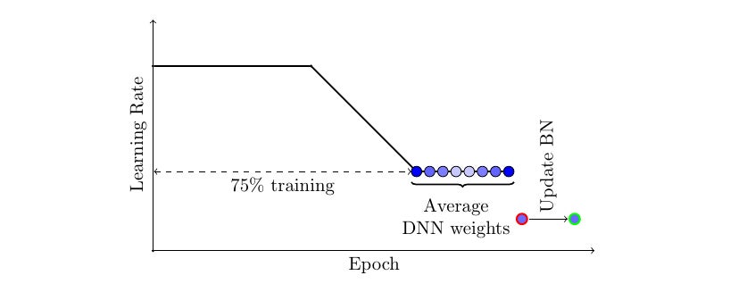
Figure 2. Illustration of the learning rate schedule adopted by SWA. Standard decaying schedule is used for the first 75% of the training and then a high constant value is used for the remaining 25%. The SWA averages are formed during the last 25% of training.
One important detail is the batch normalization. Batch normalization layers compute running statistics of activations during training. Note that the SWA averages of the weights are never used to make predictions during training. So the batch normalization layers do not have the activation statistics computed at the end of training. We can compute these statistics by doing a single forward pass on the train data with the SWA model.
While we focus on SGD for simplicity in the description above, SWA can be combined with any optimizer. You can also use cyclical learning rates instead of a high constant value (see e.g., [2]).
How to use SWA in PyTorch?
In torch.optim.swa_utils we implement all the SWA ingredients to make it convenient to use SWA with any model. In particular, we implement AveragedModel class for SWA models, SWALR learning rate scheduler, and update_bn utility function to update SWA batch normalization statistics at the end of training.
In the example below, swa_model is the SWA model that accumulates the averages of the weights. We train the model for a total of 300 epochs, and we switch to the SWA learning rate schedule and start to collect SWA averages of the parameters at epoch 160.
from torch.optim.swa_utils import AveragedModel, SWALR
from torch.optim.lr_scheduler import CosineAnnealingLR

loader, optimizer, model, loss_fn = ...
swa_model = AveragedModel(model)
scheduler = CosineAnnealingLR(optimizer, T_max=100)
swa_start = 5
swa_scheduler = SWALR(optimizer, swa_lr=0.05)

for epoch in range(100):
      for input, target in loader:
          optimizer.zero_grad()
          loss_fn(model(input), target).backward()
          optimizer.step()
      if epoch > swa_start:
          swa_model.update_parameters(model)
          swa_scheduler.step()
      else:
          scheduler.step()

# Update bn statistics for the swa_model at the end
torch.optim.swa_utils.update_bn(loader, swa_model)
# Use swa_model to make predictions on test data
preds = swa_model(test_input)
Next, we explain each component of torch.optim.swa_utils in detail.
AveragedModel class serves to compute the weights of the SWA model. You can create an averaged model by running swa_model = AveragedModel(model). You can then update the parameters of the averaged model by swa_model.update_parameters(model). By default, AveragedModel computes a running equal average of the parameters that you provide, but you can also use custom averaging functions with the avg_fn parameter. In the following example, ema_model computes an exponential moving average.
ema_avg = lambda averaged_model_parameter, model_parameter, num_averaged:\
0.1 * averaged_model_parameter + 0.9 * model_parameter
ema_model = torch.optim.swa_utils.AveragedModel(model, avg_fn=ema_avg)
In practice, we find an equal average with the modified learning rate schedule in Figure 2 provides the best performance.
SWALR is a learning rate scheduler that anneals the learning rate to a fixed value, and then keeps it constant. For example, the following code creates a scheduler that linearly anneals the learning rate from its initial value to 0.05 in 5 epochs within each parameter group.
swa_scheduler = torch.optim.swa_utils.SWALR(optimizer,
anneal_strategy="linear", anneal_epochs=5, swa_lr=0.05)
We also implement cosine annealing to a fixed value (anneal_strategy="cos"). In practice, we typically switch to SWALR at epoch swa_start (e.g. after 75% of the training epochs), and simultaneously start to compute the running averages of the weights:
scheduler = torch.optim.lr_scheduler.CosineAnnealingLR(optimizer, T_max=100)
swa_start = 75
for epoch in range(100):
      # <train epoch>
      if i > swa_start:
          swa_model.update_parameters(model)
          swa_scheduler.step()
      else:
          scheduler.step()
Finally, update_bn is a utility function that computes the batchnorm statistics for the SWA model on a given dataloader loader:
torch.optim.swa_utils.update_bn(loader, swa_model)
update_bn applies the swa_model to every element in the dataloader and computes the activation statistics for each batch normalization layer in the model.
Once you computed the SWA averages and updated the batch normalization layers, you can apply swa_model to make predictions on test data.
Why does it work?
There are large flat regions of the loss surface [9]. In Figure 3 below, we show a visualization of the loss surface in a subspace of the parameter space containing a path connecting two independently trained SGD solutions, such that the loss is similarly low at every point along the path. SGD converges near the boundary of these regions because there isn’t much gradient signal to move inside, as the points in the region all have similarly low values of loss. By increasing the learning rate, SWA spins around this flat region, and then by averaging the iterates, moves towards the center of the flat region.
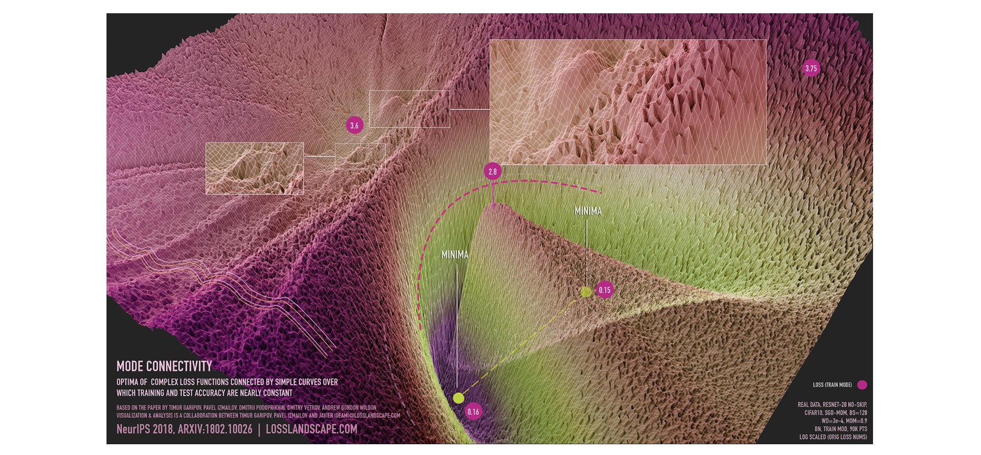
Figure 3: visualization of mode connectivity for ResNet-20 with no skip connections on CIFAR-10 dataset. The visualization is created in collaboration with Javier Ideami (https://losslandscape.com/). For more details, see this blogpost.
We expect solutions that are centered in the flat region of the loss to generalize better than those near the boundary. Indeed, train and test error surfaces are not perfectly aligned in the weight space. Solutions that are centered in the flat region are not as susceptible to the shifts between train and test error surfaces as those near the boundary. In Figure 4 below, we show the train loss and test error surfaces along the direction connecting the SWA and SGD solutions. As you can see, while the SWA solution has a higher train loss compared to the SGD solution, it is centered in a region of low loss and has a substantially better test error.
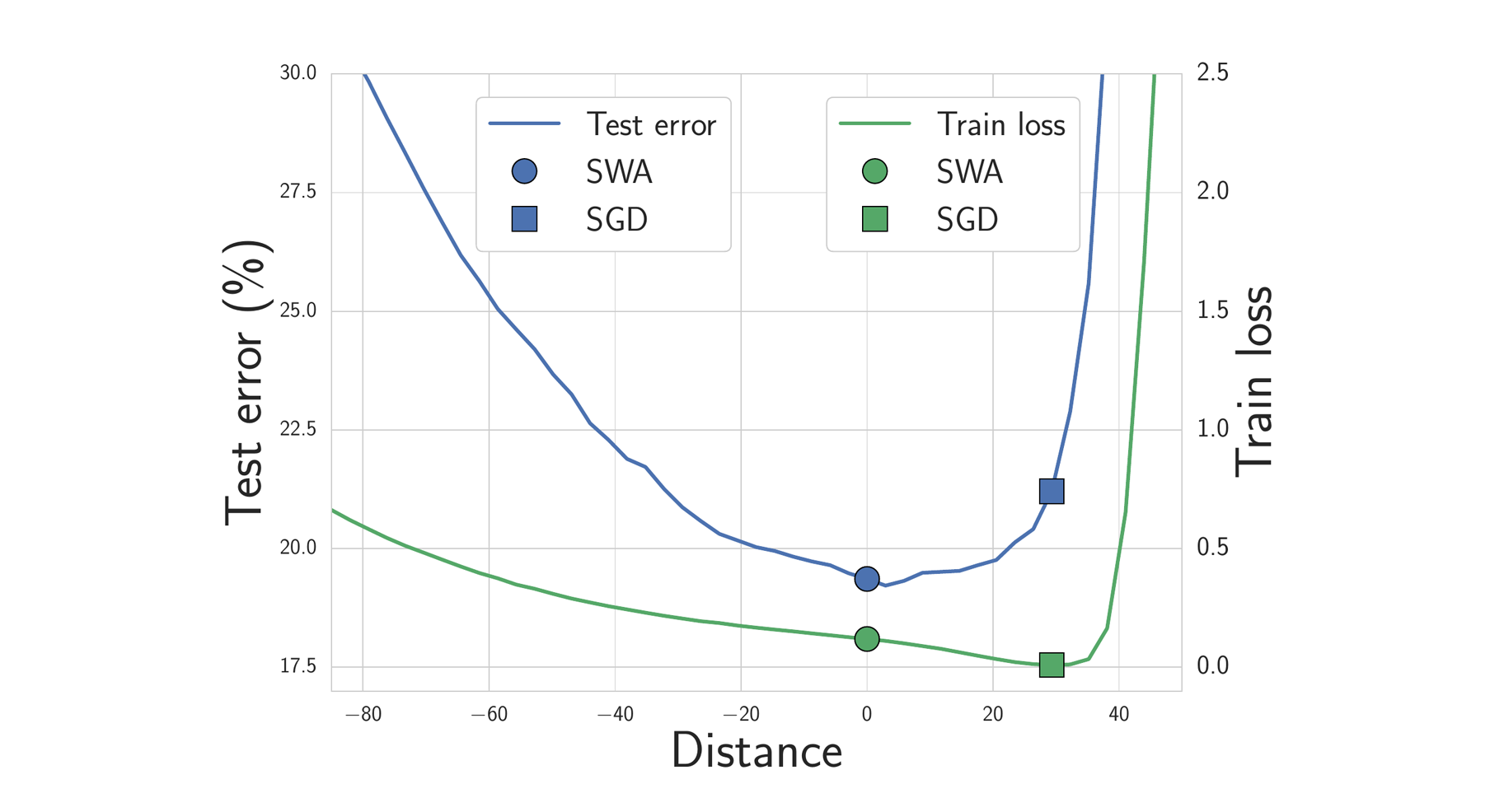
Figure 4. Train loss and test error along the line connecting the SWA solution (circle) and SGD solution (square). The SWA solution is centered in a wide region of low train loss, while the SGD solution lies near the boundary. Because of the shift between train loss and test error surfaces, the SWA solution leads to much better generalization.
What are the results achieved with SWA?
We release a GitHub repo with examples using the PyTorch implementation of SWA for training DNNs. For example, these examples can be used to achieve the following results on CIFAR-100:
| VGG-16 | ResNet-164 | WideResNet-28×10 | |
|---|---|---|---|
| SGD | 72.8 ± 0.3 | 78.4 ± 0.3 | 81.0 ± 0.3 |
| SWA | 74.4 ± 0.3 | 79.8 ± 0.4 | 82.5 ± 0.2 |
Semi-Supervised Learning
In a follow-up paper SWA was applied to semi-supervised learning, where it improved the best reported results in multiple settings [2]. For example, with SWA you can get 95% accuracy on CIFAR-10 if you only have the training labels for 4k training data points (the previous best reported result on this problem was 93.7%). This paper also explores averaging multiple times within epochs, which can accelerate convergence and find still flatter solutions in a given time.
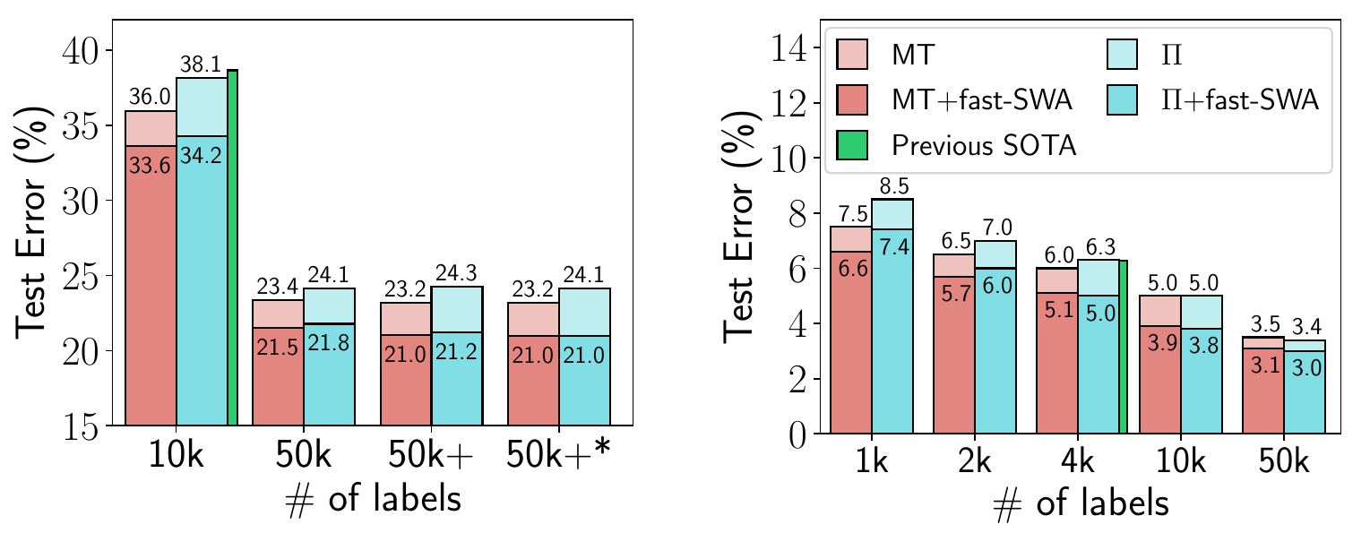
Figure 5. Performance of fast-SWA on semi-supervised learning with CIFAR-10. fast-SWA achieves record results in every setting considered.
Reinforcement Learning
In another follow-up paper SWA was shown to improve the performance of policy gradient methods A2C and DDPG on several Atari games and MuJoCo environments [3]. This application is also an instance of where SWA is used with Adam. Recall that SWA is not specific to SGD and can benefit essentially any optimizer.
| Environment Name | A2C | A2C + SWA |
|---|---|---|
| Breakout | 522 ± 34 | 703 ± 60 |
| Qbert | 18777 ± 778 | 21272 ± 655 |
| SpaceInvaders | 7727 ± 1121 | 21676 ± 8897 |
| Seaquest | 1779 ± 4 | 1795 ± 4 |
| BeamRider | 9999 ± 402 | 11321 ± 1065 |
| CrazyClimber | 147030 ± 10239 | 139752 ± 11618 |
Low Precision Training
We can filter through quantization noise by combining weights that have been rounded down with weights that have been rounded up. Moreover, by averaging weights to find a flat region of the loss surface, large perturbations of the weights will not affect the quality of the solution (Figures 9 and 10). Recent work shows that by adapting SWA to the low precision setting, in a method called SWALP, one can match the performance of full-precision SGD even with all training in 8 bits [5]. This is quite a practically important result, given that (1) SGD training in 8 bits performs notably worse than full precision SGD, and (2) low precision training is significantly harder than predictions in low precision after training (the usual setting). For example, a ResNet-164 trained on CIFAR-100 with float (16-bit) SGD achieves 22.2% error, while 8-bit SGD achieves 24.0% error. By contrast, SWALP with 8 bit training achieves 21.8% error.
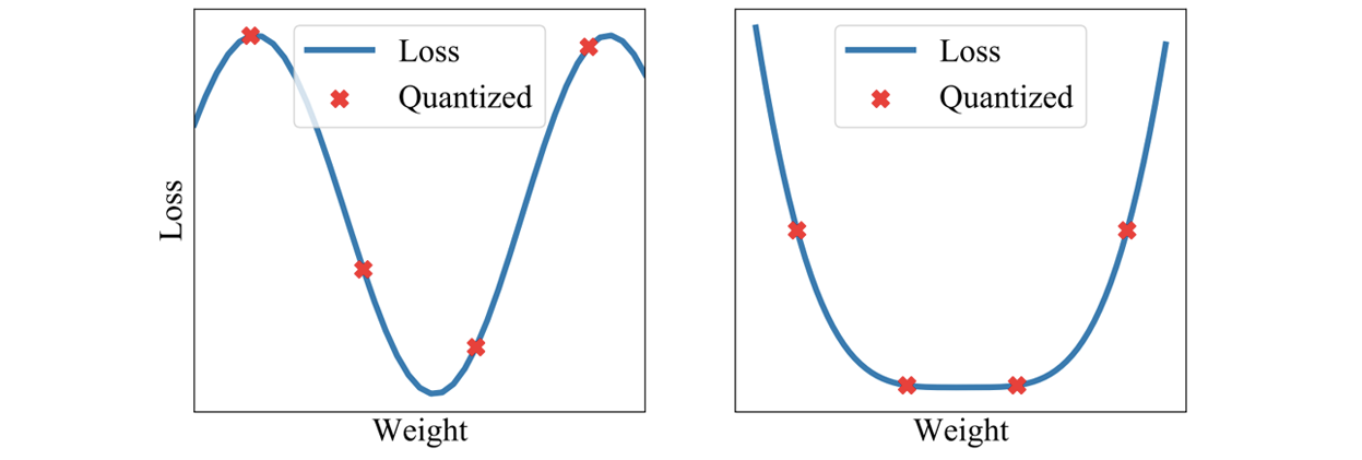
Figure 9. Quantizing a solution leads to a perturbation of the weights which has a greater effect on the quality of the sharp solution (left) compared to wide solution (right).
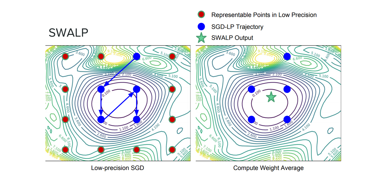
Figure 10. The difference between standard low precision training and SWALP.
Another work, SQWA, presents an approach for quantization and fine-tuning of neural networks in low precision [12]. In particular, SQWA achieved state-of-the-art results for DNNs quantized to 2 bits on CIFAR-100 and ImageNet.
Calibration and Uncertainty Estimates
By finding a centred solution in the loss, SWA can also improve calibration and uncertainty representation. Indeed, SWA can be viewed as an approximation to an ensemble, resembling a Bayesian model average, but with a single model [1].
SWA can be viewed as taking the first moment of SGD iterates with a modified learning rate schedule. We can directly generalize SWA by also taking the second moment of iterates to form a Gaussian approximate posterior over the weights, further characterizing the loss geometry with SGD iterates. This approach,SWA-Gaussian (SWAG) is a simple, scalable and convenient approach to uncertainty estimation and calibration in Bayesian deep learning [4]. The SWAG distribution approximates the shape of the true posterior: Figure 6 below shows the SWAG distribution and the posterior log-density for ResNet-20 on CIFAR-10.
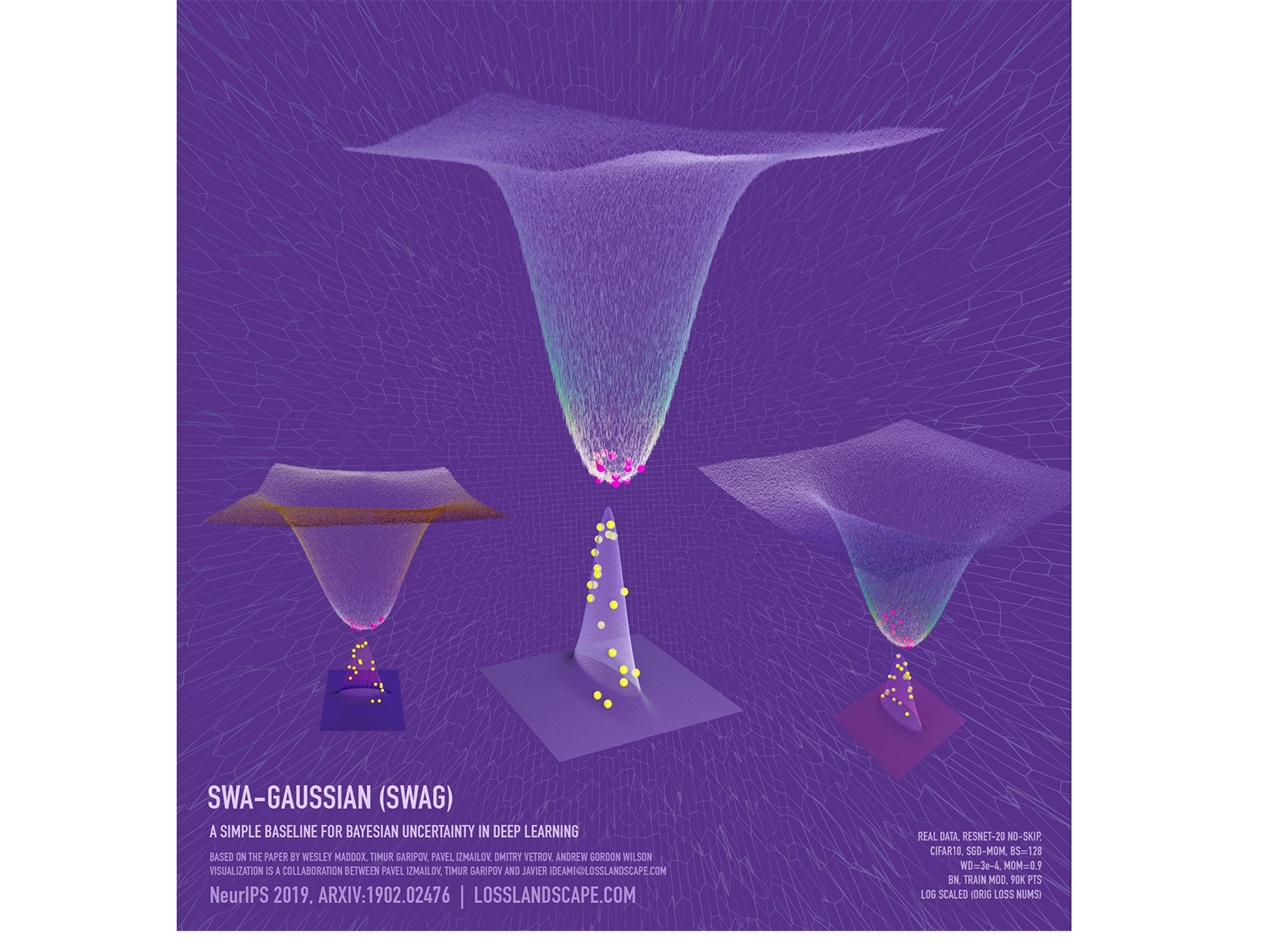
Figure 6. SWAG posterior approximation and the loss surface for a ResNet-20 without skip-connections trained on CIFAR-10 in the subspace formed by the two largest eigenvalues of the SWAG covariance matrix. The shape of SWAG distribution is aligned with the posterior: the peaks of the two distributions coincide, and both distributions are wider in one direction than in the orthogonal direction. Visualization created in collaboration with Javier Ideami.
Empirically, SWAG performs on par or better than popular alternatives including MC dropout, KFAC Laplace, and temperature scaling on uncertainty quantification, out-of-distribution detection, calibration and transfer learning in computer vision tasks. Code for SWAG is available here.
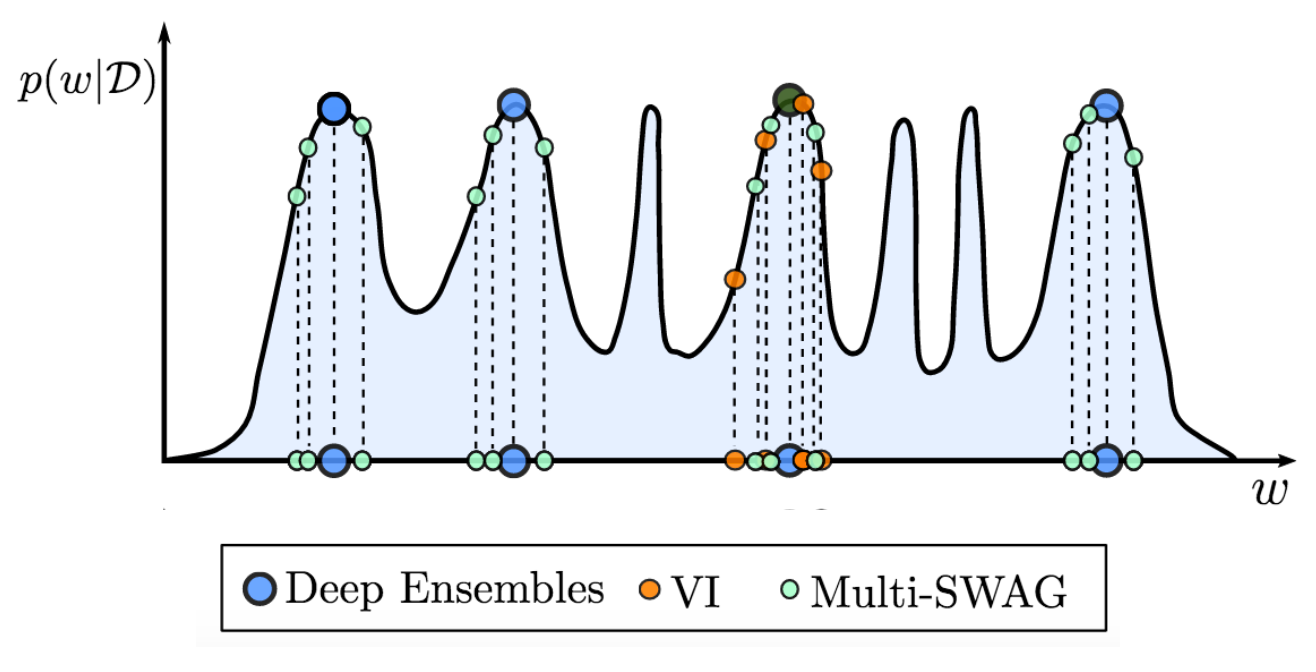
Figure 7. MultiSWAG generalizes SWAG and deep ensembles, to perform Bayesian model averaging over multiple basins of attraction, leading to significantly improved performance. By contrast, as shown here, deep ensembles select different modes, while standard variational inference (VI) marginalizes (model averages) within a single basin.
MultiSWAG [9] uses multiple independent SWAG models to form a mixture of Gaussians as an approximate posterior distribution. Different basins of attraction contain highly complementary explanations of the data. Accordingly, marginalizing over these multiple basins provides a significant boost in accuracy and uncertainty representation. MultiSWAG can be viewed as a generalization of deep ensembles, but with performance improvements.
Indeed, we see in Figure 8 that MultiSWAG entirely mitigates double descent – more flexible models have monotonically improving performance – and provides significantly improved generalization over SGD. For example, when the ResNet-18 has layers of width 20, Multi-SWAG achieves under 30% error whereas SGD achieves over 45%, more than a 15% gap!
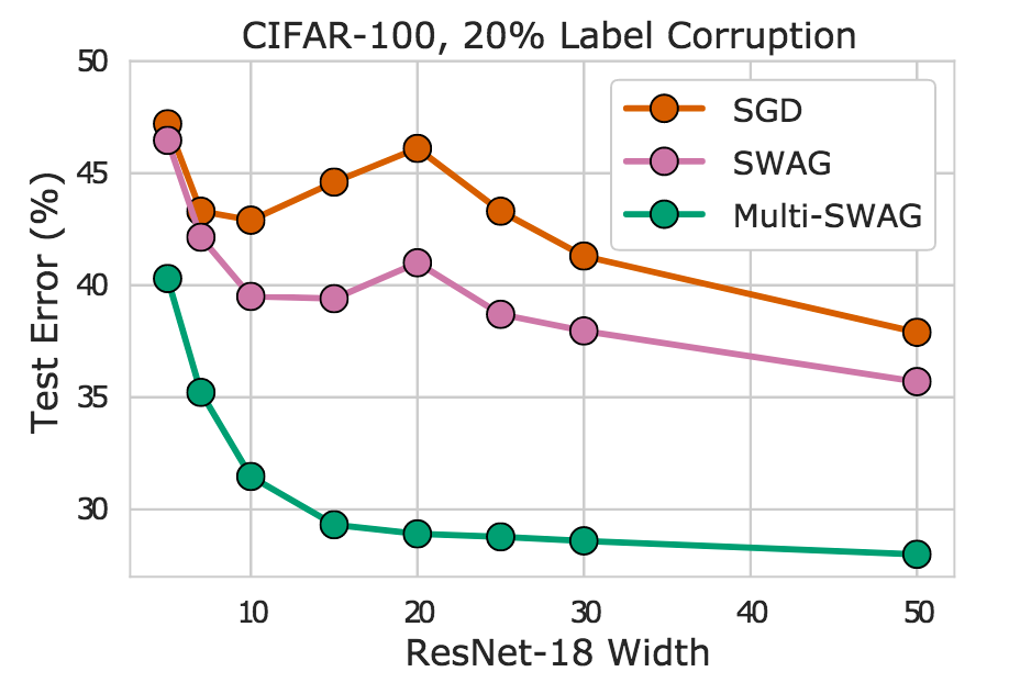
Figure 8. SGD, SWAG, and Multi-SWAG on CIFAR-100 for a ResNet-18 with varying widths. We see Multi-SWAG in particular mitigates double descent and provides significant accuracy improvements over SGD.
Reference [10] also considers Multi-SWA, which uses multiple independently trained SWA solutions in an ensemble, providing performance improvements over deep ensembles without any additional computational cost. Code for MultiSWA and MultiSWAG is available here.
Another method, Subspace Inference, constructs a low-dimensional subspace around the SWA solution and marginalizes the weights in this subspace to approximate the Bayesian model average [5]. Subspace Inference uses the statistics from the SGD iterates to construct both the SWA solution and the subspace. The method achieves strong performance in terms of prediction accuracy and uncertainty calibration both in classification and regression problems. Code is available here.
Try it Out!
One of the greatest open questions in deep learning is why SGD manages to find good solutions, given that the training objectives are highly multimodal, and there are many settings of parameters that achieve no training loss but poor generalization. By understanding geometric features such as flatness, which relate to generalization, we can begin to resolve these questions and build optimizers that provide even better generalization, and many other useful features, such as uncertainty representation. We have presented SWA, a simple drop-in replacement for standard optimizers such as SGD and Adam, which can in principle, benefit anyone training a deep neural network. SWA has been demonstrated to have a strong performance in several areas, including computer vision, semi-supervised learning, reinforcement learning, uncertainty representation, calibration, Bayesian model averaging, and low precision training.
We encourage you to try out SWA! SWA is now as easy as any standard training in PyTorch. And even if you have already trained your model, you can use SWA to significantly improve performance by running it for a small number of epochs from a pre-trained model.
[1] Averaging Weights Leads to Wider Optima and Better Generalization; Pavel Izmailov, Dmitry Podoprikhin, Timur Garipov, Dmitry Vetrov, Andrew Gordon Wilson; Uncertainty in Artificial Intelligence (UAI), 2018.
[2] There Are Many Consistent Explanations of Unlabeled Data: Why You Should Average; Ben Athiwaratkun, Marc Finzi, Pavel Izmailov, Andrew Gordon Wilson; International Conference on Learning Representations (ICLR), 2019.
[3] Improving Stability in Deep Reinforcement Learning with Weight Averaging; Evgenii Nikishin, Pavel Izmailov, Ben Athiwaratkun, Dmitrii Podoprikhin, Timur Garipov, Pavel Shvechikov, Dmitry Vetrov, Andrew Gordon Wilson; UAI 2018 Workshop: Uncertainty in Deep Learning, 2018.
[4] A Simple Baseline for Bayesian Uncertainty in Deep Learning Wesley Maddox, Timur Garipov, Pavel Izmailov, Andrew Gordon Wilson; Neural Information Processing Systems (NeurIPS), 2019.
[5] Subspace Inference for Bayesian Deep Learning Pavel Izmailov, Wesley Maddox, Polina Kirichenko, Timur Garipov, Dmitry Vetrov, Andrew Gordon Wilson Uncertainty in Artificial Intelligence (UAI), 2019.
[6] SWALP : Stochastic Weight Averaging in Low Precision Training Guandao Yang, Tianyi Zhang, Polina Kirichenko, Junwen Bai, Andrew Gordon Wilson, Christopher De Sa; International Conference on Machine Learning (ICML), 2019.
[7] David Ruppert. Efficient estimations from a slowly convergent Robbins-Monro process; Technical report, Cornell University Operations Research and Industrial Engineering, 1988.
[8] Acceleration of stochastic approximation by averaging. Boris T Polyak and Anatoli B Juditsky; SIAM Journal on Control and Optimization, 30(4):838–855, 1992.
[9] Loss Surfaces, Mode Connectivity, and Fast Ensembling of DNNs Timur Garipov, Pavel Izmailov, Dmitrii Podoprikhin, Dmitry Vetrov, Andrew Gordon Wilson. Neural Information Processing Systems (NeurIPS), 2018.
[10] Bayesian Deep Learning and a Probabilistic Perspective of Generalization Andrew Gordon Wilson, Pavel Izmailov. ArXiv preprint, 2020.
[11] Stochastic Weight Averaging in Parallel: Large-Batch Training That Generalizes Well Gupta, Vipul, Santiago Akle Serrano, and Dennis DeCoste; International Conference on Learning Representations (ICLR). 2019.
[12] SQWA: Stochastic Quantized Weight Averaging for Improving the Generalization Capability of Low-Precision Deep Neural Networks Shin, Sungho, Yoonho Boo, and Wonyong Sung; arXiv preprint 2020.