Overview of PyTorch Autograd Engine

by Preferred Networks, Inc.

This blog post is based on PyTorch version 1.8, although it should apply for older versions too, since most of the mechanics have remained constant.

To help understand the concepts explained here, it is recommended that you read the awesome blog post by @ezyang: PyTorch internals if you are not familiar with PyTorch architecture components such as ATen or c10d.

What is autograd?

Background

PyTorch computes the gradient of a function with respect to the inputs by using automatic differentiation. Automatic differentiation is a technique that, given a computational graph, calculates the gradients of the inputs. Automatic differentiation can be performed in two different ways; forward and reverse mode. Forward mode means that we calculate the gradients along with the result of the function, while reverse mode requires us to evaluate the function first, and then we calculate the gradients starting from the output. While both modes have their pros and cons, the reverse mode is the de-facto choice since the number of outputs is smaller than the number of inputs, which allows a much more efficient computation. Check [3] to learn more about this.

Automatic differentiation relies on a classic calculus formula known as the chain-rule. The chain rule allows us to calculate very complex derivatives by splitting them and recombining them later.

Formally speaking, given a composite function $f(g(x))$ , we can calculate its derivative as $\frac{\partial}{\partial x} f(g(x)) = f'(g(x))g'(x)$ . This result is what makes automatic differentiation work. By combining the derivatives of the simpler functions that compose a larger one, such as a neural network, it is possible to compute the exact value of the gradient at a given point rather than relying on the numerical approximation, which would require multiple perturbations in the input to obtain a value.

To get the intuition of how the reverse mode works, let’s look at a simple function $f(x, y) = log(x*y)$ . Figure 1 shows its computational graph where the inputs x, y in the left, flow through a series of operations to generate the output z.

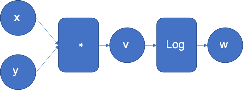
Figure 1: Computational graph of f(x, y) = log(x*y)

The automatic differentiation engine will normally execute this graph. It will also extend it to calculate the derivatives of w with respect to the inputs x, y, and the intermediate result v.

The example function can be decomposed in f and g, where $f(x, y) = log(g(x, y))$ and $g(x, y) = xy$ . Every time the engine executes an operation in the graph, the derivative of that operation is added to the graph to be executed later in the backward pass. Note, that the engine knows the derivatives of the basic functions.

In the example above, when multiplying x and y to obtain v, the engine will extend the graph to calculate the partial derivatives of the multiplication by using the multiplication derivative definition that it already knows. $\frac{\partial}{\partial x} g(x, y) = y$ and $\frac{\partial}{\partial y} g(x, y) = x$ . The resulting extended graph is shown in Figure 2, where the MultDerivative node also calculates the product of the resulting gradients by an input gradient to apply the chain rule; this will be explicitly seen in the following operations. Note that the backward graph (green nodes) will not be executed until all the forward steps are completed.

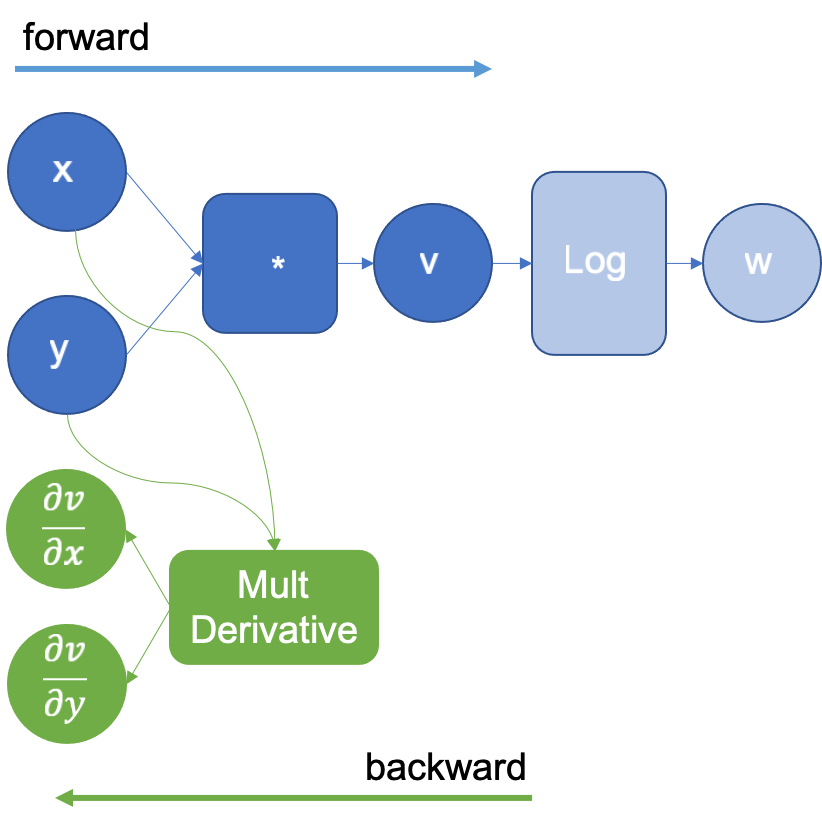
Figure 2: Computational graph extended after executing the logarithm

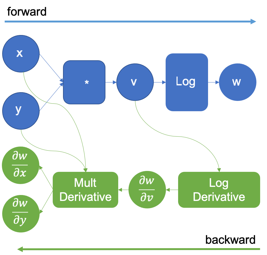
Continuing, the engine now calculates the $log(v)$ operation and extends the graph again with the log derivative that it knows to be $\frac{1}{v}$ . This is shown in figure 3. This operation generates the result $\frac{\partial w}{\partial v}$ that when propagated backward and multiplied by the multiplication derivative as in the chain rule, generates the derivatives $\frac{\partial w}{\partial x}$ , $\frac{\partial w}{\partial y}$ .

Figure 3: Computational graph extended after executing the logarithm

The original computation graph is extended with a new dummy variable z that is the same w. The derivative of z with respect to w is 1 as they are the same variable, this trick allows us to apply the chain rule to calculate the derivatives of the inputs. After the forward pass is complete, we start the backward pass, by supplying the initial value of 1.0 for $\frac{\partial z}{\partial w}$ . This is shown in Figure 4.

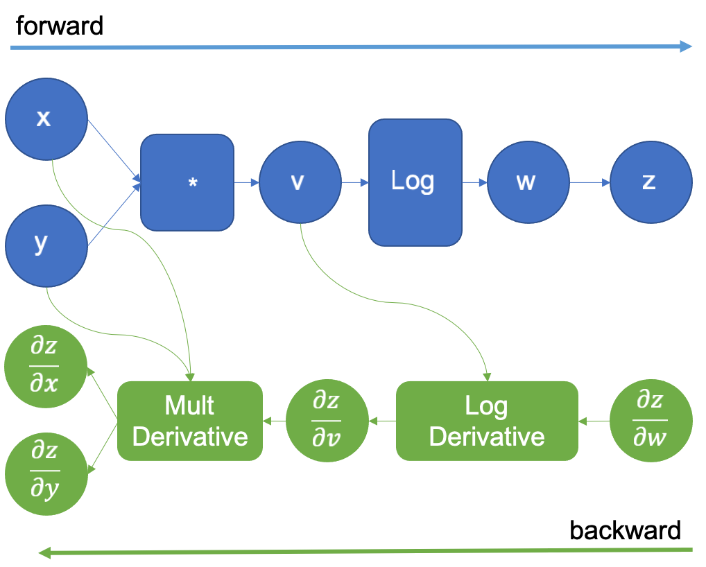
Figure 4: Computational graph extended for reverse auto differentiation

Then following the green graph we execute the LogDerivative operation $\frac{1}{v}$ that the auto differentiation engine introduced, and multiply its result by $\frac{\partial z}{\partial w}$ to obtain the gradient $\frac{\partial z}{\partial v}$ as per the chain rule states. Next, the multiplication derivative is executed in the same way, and the desired derivatives $\frac{\partial z}{\partial x} \frac{\partial z}{\partial y}$ are finally obtained.

Formally, what we are doing here, and PyTorch autograd engine also does, is computing a Jacobian-vector product (Jvp) to calculate the gradients of the model parameters, since the model parameters and inputs are vectors.

The Jacobian-vector product

When we calculate the gradient of a vector-valued function $f(\overline{x}) = \overline{y}$ (a function whose inputs and outputs are vectors), we are essentially constructing a Jacobian matrix .

Thanks to the chain rule, multiplying the Jacobian matrix of a function $f(\overline{x}) = \overline{y}$ by a vector $v$ with the previously calculated gradients of a scalar function $z = g(\overline{y})$ results in the gradients $\frac{\partial z}{\partial x_1} \cdots \frac{\partial z}{\partial x_n}$ of the scalar output with respect to the vector-valued function inputs.

As an example, let’s look at some functions in python notation to show how the chain rule applies.

$f(x_1, x_2) = (log(x_1 x_2), sin(x_2))$

def f(x1, x2):
      a = x1 * x2
      y1 = log(a)
      y2 = sin(x2)
      return (y1, y2)

$g(y_1, y_2) = y_1 y_2$

def g(y1, y2):
      return y1 * y2

Now, if we derive this by hand using the chain rule and the definition of the derivatives, we obtain the following set of identities that we can directly plug into the Jacobian matrix of $f(x_1, x_2)$

$\frac{\partial y_1}{\partial x_1} = \frac{\partial y_1}{\partial a}\frac{\partial a}{\partial x_1} = \frac{1}{x_1}$

$\frac{\partial y_1}{\partial x_2} = \frac{\partial y_1}{\partial a}\frac{\partial a}{\partial x_2} = \frac{1}{x_2}$

$\frac{\partial y_2}{\partial x_1} = 0$

$\frac{\partial y_2}{\partial x_2} = cos(x_2)$

Next, let’s consider the gradients for the scalar function $z = g(y_1, y_2)$

$\frac{\partial z}{y_1} = y_2$

$\frac{\partial z}{y_2} = y_1$

If we now calculate the transpose-Jacobian vector product obeying the chain rule, we obtain the following expression:

$\begin{pmatrix}\frac{\partial y_1}{\partial x_1} & \frac{\partial y_1}{\partial x_2} \\\\ \frac{\partial y_2}{\partial x_1} & \frac{\partial y_2}{\partial x_2} \end{pmatrix}^{t} \begin{pmatrix} y_2\\y_1 \end{pmatrix} = \begin{pmatrix}\frac{1}{x_1} & \frac{1}{x_2} \\\\ 0 & cos(x_2)) \end{pmatrix}^{t} \begin{pmatrix} y_2\\y_1 \end{pmatrix} = \begin{pmatrix} \frac{1}{x_1}y_2\\\frac{1}{x_2}y_2+cos(x_2)y_1 \end{pmatrix}$

Evaluating the Jvp for $(x_1, x_2) = (0.5, 0.75)$ yields the result: $(\frac{dy}{x_1}, \frac{dy}{x_2}) = (1.3633, 0.1912)$ We can execute the same expression in PyTorch and calculate the gradient of the input:

>>> import torch

>>> x = torch.tensor([0.5, 0.75], requires_grad=True)

>>> y = torch.log(x[0] * x[1]) * torch.sin(x[1])

>>> y.backward(1.0)

>>> x.grad

tensor([1.3633, 0.1912])

The result is the same as our hand-calculated Jacobian-vector product! However, PyTorch never constructed the matrix as it could grow prohibitively large but instead, created a graph of operations that traversed backward while applying the Jacobian-vector products defined in tools/autograd/derivatives.yaml.

Going through the graph

Every time PyTorch executes an operation, the autograd engine constructs the graph to be traversed backward. The reverse mode auto differentiation starts by adding a scalar variable at the end $z = w$ so that $\frac{\partial z}{\partial w} = 1$ as we saw in the introduction. This is the initial gradient value that is supplied to the Jvp engine calculation as we saw in the section above.

In PyTorch, the initial gradient is explicitly set by the user when he calls the backward method.

Then, the Jvp calculation starts but it never constructs the matrix. Instead, when PyTorch records the computational graph, the derivatives of the executed forward operations are added (Backward Nodes). Figure 5 shows a backward graph generated by the execution of the functions $f(x_1, x_2)$ and $g(y_1, y_2)$ seen before.

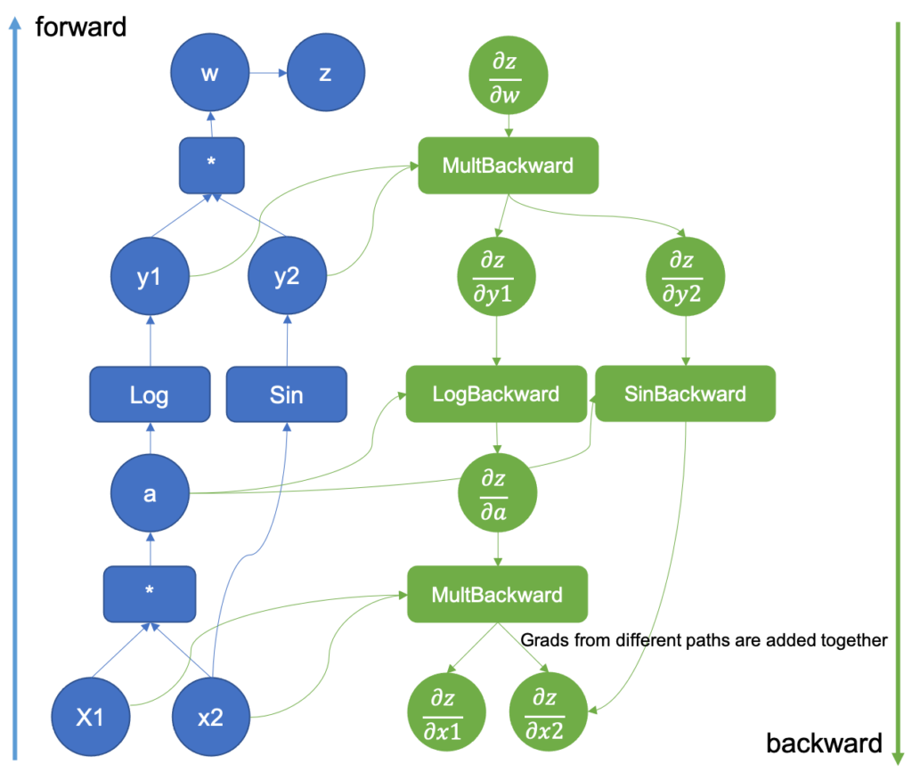
Figure 5: Computational Graph extended with the backward pass

Once the forward pass is done, the results are used in the backward pass where the derivatives in the computational graph are executed. The basic derivatives are stored in the tools/autograd/derivatives.yaml file and they are not regular derivatives but the Jvp versions of them [3]. They take their primitive function inputs and outputs as parameters along with the gradient of the function outputs with respect to the final outputs. By repeatedly multiplying the resulting gradients by the next Jvp derivatives in the graph, the gradients up to the inputs will be generated following the chain rule.

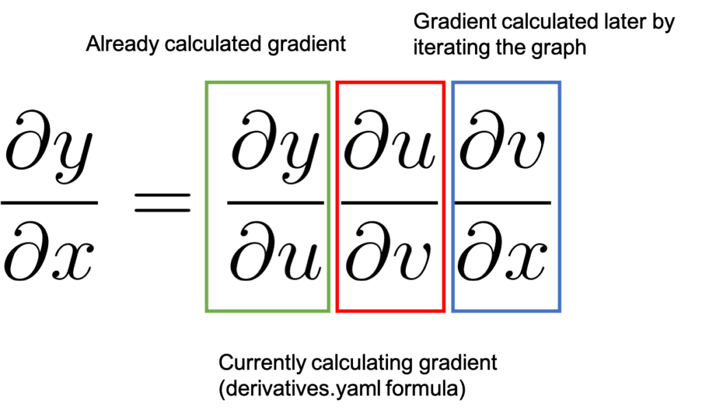
Figure 6: How the chain rule is applied in backward differentiation

Figure 6 represents the process by showing the chain rule. We started with a value of 1.0 as detailed before which is the already calculated gradient $\frac{\partial y}{\partial u}$ highlighted in green. And we move to the next node in the graph. The backward function registered in derivatives.yaml will calculate the associated $\frac{\partial u}{\partial v}$ value highlighted in red and multiply it by $\frac{\partial y}{\partial u}$ . By the chain rule this results in $\frac{\partial y}{\partial v}$ which will be the already calculated gradient (green) when we process the next backward node in the graph.

You may also have noticed that in Figure 5 there is a gradient generated from two different sources. When two different functions share an input, the gradients with respect to the output are aggregated for that input, and calculations using that gradient can’t proceed unless all the paths have been aggregated together.

Let’s see an example of how the derivatives are stored in PyTorch.

Suppose that we are currently processing the backward propagation of the $log$ function, in the LogBackward node in Figure 2. The derivative of $log$ in derivatives.yaml is specified as grad.div(self.conj()). grad is the already calculated gradient $\frac{\partial z}{\partial y1}$ and self.conj() is the complex conjugate of the input vector. For complex numbers PyTorch calculates a special derivative called the conjugate Wirtinger derivative [6]. This derivative takes the complex number and its conjugate and by operating some magic that is described in [6], they are the direction of steepest descent when plugged into optimizers.

This code translates to $(\frac{\partial z}{\partial y1} \frac{1}{v})$ , the corresponding green, and red squares in Figure 3. Continuing, the autograd engine will execute the next operation; backward of the multiplication. As before, the inputs are the original function’s inputs and the gradient calculated from the $log$ backward step. This step will keep repeating until we reach the gradient with respect to the inputs and the computation will be finished. The gradient of $\frac{\partial z}{x2}$ is only completed once the multiplication and sin gradients are added together. As you can see, we computed the equivalent of the Jvp but without constructing the matrix.

In the next post we will dive inside PyTorch code to see how this graph is constructed and where are the relevant pieces should you want to experiment with it!

References

Recommended: shows why the backprop is formally expressed with the Jacobian

https://cs.ubc.ca/~fwood/CS340/lectures/AD1.pdf

Overview of PyTorch Autograd Engine

What is autograd?

References

Docs

Tutorials

Resources