This week, we officially released PyTorch 1.1, a large feature update to PyTorch 1.0. One of the new features we’ve added is better support for fast, custom Recurrent Neural Networks (fastrnns) with TorchScript (the PyTorch JIT) (https://pytorch.org/docs/stable/jit.html).
RNNs are popular models that have shown good performance on a variety of NLP tasks that come in different shapes and sizes. PyTorch implements a number of the most popular ones, the Elman RNN, GRU, and LSTM as well as multi-layered and bidirectional variants.
However, many users want to implement their own custom RNNs, taking ideas from recent literature. Applying Layer Normalization to LSTMs is one such use case. Because the PyTorch CUDA LSTM implementation uses a fused kernel, it is difficult to insert normalizations or even modify the base LSTM implementation. Many users have turned to writing custom implementations using standard PyTorch operators, but such code suffers from high overhead: most PyTorch operations launch at least one kernel on the GPU and RNNs generally run many operations due to their recurrent nature. However, we can apply TorchScript to fuse operations and optimize our code automatically, launching fewer, more optimized kernels on the GPU.
Our goal is for users to be able to write fast, custom RNNs in TorchScript without writing specialized CUDA kernels to achieve similar performance. In this post, we’ll provide a tutorial for how to write your own fast RNNs with TorchScript. To better understand the optimizations TorchScript applies, we’ll examine how those work on a standard LSTM implementation but most of the optimizations can be applied to general RNNs.
Writing custom RNNs
To get started, you can use this file as a template to write your own custom RNNs.
We are constantly improving our infrastructure on trying to make the performance better. If you want to gain the speed/optimizations that TorchScript currently provides (like operator fusion, batch matrix multiplications, etc.), here are some guidelines to follow. The next section explains the optimizations in depth.
- If the customized operations are all element-wise, that’s great because you can get the benefits of the PyTorch JIT’s operator fusion automatically!
- If you have more complex operations (e.g. reduce ops mixed with element-wise ops), consider grouping the reduce operations and element-wise ops separately in order to fuse the element-wise operations into a single fusion group.
- If you want to know about what has been fused in your custom RNN, you can inspect the operation’s optimized graph by using
graph_for. UsingLSTMCellas an example:
# get inputs and states for LSTMCell

 inputs = get_lstm_inputs()

 # instantiate a ScriptModule

 cell = LSTMCell(input_size, hidden_size)

 # print the optimized graph using graph_for

 out = cell(inputs)
 print(cell.graph_for(inputs))
This will generate the optimized TorchScript graph (a.k.a PyTorch JIT IR) for the specialized inputs that you provides:
graph(%x : Float(*, *),
         %hx : Float(*, *),
         %cx : Float(*, *),
         %w_ih : Float(*, *),
         %w_hh : Float(*, *),
         %b_ih : Float(*),
         %b_hh : Float(*)):
     %hy : Float(*, *), %cy : Float(*, *) = prim::DifferentiableGraph_0(%cx, %b_hh, %b_ih, %hx, %w_hh, %x, %w_ih)
     %30 : (Float(*, *), Float(*, *)) = prim::TupleConstruct(%hy, %cy)
     return (%30)
     with prim::DifferentiableGraph_0 = graph(%13 : Float(*, *),
         %29 : Float(*),
         %33 : Float(*),
         %40 : Float(*, *),
         %43 : Float(*, *),
         %45 : Float(*, *),
         %48 : Float(*, *)):
     %49 : Float(*, *) = aten::t(%48)
     %47 : Float(*, *) = aten::mm(%45, %49)
     %44 : Float(*, *) = aten::t(%43)
     %42 : Float(*, *) = aten::mm(%40, %44)
     ...some broadcast sizes operations...
     %hy : Float(*, *), %287 : Float(*, *), %cy : Float(*, *), %outgate.1 : Float(*, *), %cellgate.1 : Float(*, *), %forgetgate.1 : Float(*, *), %ingate.1 : Float(*, *) = prim::FusionGroup_0(%13, %346, %345, %344, %343)
     ...some broadcast sizes operations...
     return (%hy, %cy, %49, %44, %196, %199, %340, %192, %325, %185, %ingate.1, %forgetgate.1, %cellgate.1, %outgate.1, %395, %396, %287)
     with prim::FusionGroup_0 = graph(%13 : Float(*, *),
         %71 : Tensor,
         %76 : Tensor,
         %81 : Tensor,
         %86 : Tensor):
     ...some chunks, constants, and add operations...
     %ingate.1 : Float(*, *) = aten::sigmoid(%38)
     %forgetgate.1 : Float(*, *) = aten::sigmoid(%34)
     %cellgate.1 : Float(*, *) = aten::tanh(%30)
     %outgate.1 : Float(*, *) = aten::sigmoid(%26)
     %14 : Float(*, *) = aten::mul(%forgetgate.1, %13)
     %11 : Float(*, *) = aten::mul(%ingate.1, %cellgate.1)
     %cy : Float(*, *) = aten::add(%14, %11, %69)
     %4 : Float(*, *) = aten::tanh(%cy)
     %hy : Float(*, *) = aten::mul(%outgate.1, %4)
     return (%hy, %4, %cy, %outgate.1, %cellgate.1, %forgetgate.1, %ingate.1)
From the above graph we can see that it has a prim::FusionGroup_0 subgraph that is fusing all element-wise operations in LSTMCell (transpose and matrix multiplication are not element-wise ops). Some graph nodes might be hard to understand in the first place but we will explain some of them in the optimization section, we also omitted some long verbose operators in this post that is there just for correctness.
Variable-length sequences best practices
TorchScript does not support PackedSequence. Generally, when one is handling variable-length sequences, it is best to pad them into a single tensor and send that tensor through a TorchScript LSTM. Here’s an example:
sequences = [...] # List[Tensor], each Tensor is T' x C
padded = torch.utils.rnn.pad_sequence(sequences)
lengths = [seq.size(0) for seq in sequences]
padded  # T x N x C, where N is batch size and T is the max of all T'

model = LSTM(...)
output, hiddens = model(padded)
output  # T x N x C
Of course, output may have some garbage data in the padded regions; use lengths to keep track of which part you don’t need.
Optimizations
We will now explain the optimizations performed by the PyTorch JIT to speed up custom RNNs. We will use a simple custom LSTM model in TorchScript to illustrate the optimizations, but many of these are general and apply to other RNNs.
To illustrate the optimizations we did and how we get benefits from those optimizations, we will run a simple custom LSTM model written in TorchScript (you can refer the code in the custom_lstm.py or the below code snippets) and time our changes.
We set up the environment in a machine equipped with 2 Intel Xeon chip and one Nvidia P100, with cuDNN v7.3, CUDA 9.2 installed. The basic set up for the LSTM model is as follows:
input_size = 512
hidden_size = 512
mini_batch = 64
numLayers = 1
seq_length = 100
The most important thing PyTorch JIT did is to compile the python program to a PyTorch JIT IR, which is an intermediate representation used to model the program’s graph structure. This IR can then benefit from whole program optimization, hardware acceleration and overall has the potential to provide large computation gains. In this example, we run the initial TorchScript model with only compiler optimization passes that are provided by the JIT, including common subexpression elimination, constant pooling, constant propagation, dead code elimination and some peephole optimizations. We run the model training for 100 times after warm up and average the training time. The initial results for model forward time is around 27ms and backward time is around 64ms, which is a bit far away from what PyTorch cuDNN LSTM provided. Next we will explain the major optimizations we did on how we improve the performance on training or inferencing, starting with LSTMCell and LSTMLayer, and some misc optimizations.
LSTM Cell (forward)
Almost all the computations in an LSTM happen in the LSTMCell, so it’s important for us to take a look at the computations it contains and how can we improve their speed. Below is a sample LSTMCell implementation in TorchScript:
class LSTMCell(jit.ScriptModule):
    def __init__(self, input_size, hidden_size):
        super(LSTMCell, self).__init__()
        self.input_size = input_size
        self.hidden_size = hidden_size
        self.weight_ih = Parameter(torch.randn(4 * hidden_size, input_size))
        self.weight_hh = Parameter(torch.randn(4 * hidden_size, hidden_size))
        self.bias_ih = Parameter(torch.randn(4 * hidden_size))
        self.bias_hh = Parameter(torch.randn(4 * hidden_size))

    @jit.script_method
    def forward(self, input, state):
        # type: (Tensor, Tuple[Tensor, Tensor]) -> Tuple[Tensor, Tuple[Tensor, Tensor]]
        hx, cx = state
        gates = (torch.mm(input, self.weight_ih.t()) + self.bias_ih +
                 torch.mm(hx, self.weight_hh.t()) + self.bias_hh)
        ingate, forgetgate, cellgate, outgate = gates.chunk(4, 1)

        ingate = torch.sigmoid(ingate)
        forgetgate = torch.sigmoid(forgetgate)
        cellgate = torch.tanh(cellgate)
        outgate = torch.sigmoid(outgate)

        cy = (forgetgate * cx) + (ingate * cellgate)
        hy = outgate * torch.tanh(cy)

        return hy, (hy, cy)
This graph representation (IR) that TorchScript generated enables several optimizations and scalable computations. In addition to the typical compiler optimizations that we could do (CSE, constant propagation, etc. ) we can also run other IR transformations to make our code run faster.
- Element-wise operator fusion. PyTorch JIT will automatically fuse element-wise ops, so when you have adjacent operators that are all element-wise, JIT will automatically group all those operations together into a single FusionGroup, this FusionGroup can then be launched with a single GPU/CPU kernel and performed in one pass. This avoids expensive memory reads and writes for each operation.
- Reordering chunks and pointwise ops to enable more fusion. An LSTM cell adds gates together (a pointwise operation), and then chunks the gates into four pieces: the ifco gates. Then, it performs pointwise operations on the ifco gates like above. This leads to two fusion groups in practice: one fusion group for the element-wise ops pre-chunk, and one group for the element-wise ops post-chunk. The interesting thing to note here is that pointwise operations commute with
torch.chunk: Instead of performing pointwise ops on some input tensors and chunking the output, we can chunk the input tensors and then perform the same pointwise ops on the output tensors. By moving the chunk to before the first fusion group, we can merge the first and second fusion groups into one big group.

- Tensor creation on the CPU is expensive, but there is ongoing work to make it faster. At this point, a LSTMCell runs three CUDA kernels: two
gemmkernels and one for the single pointwise group. One of the things we noticed was that there was a large gap between the finish of the secondgemmand the start of the single pointwise group. This gap was a period of time when the GPU was idling around and not doing anything. Looking into it more, we discovered that the problem was thattorch.chunkconstructs new tensors and that tensor construction was not as fast as it could be. Instead of constructing new Tensor objects, we taught the fusion compiler how to manipulate a data pointer and strides to do thetorch.chunkbefore sending it into the fused kernel, shrinking the amount of idle time between the second gemm and the launch of the element-wise fusion group. This give us around 1.2x increase speed up on the LSTM forward pass.
By doing the above tricks, we are able to fuse the almost all LSTMCell forward graph (except the two gemm kernels) into a single fusion group, which corresponds to the prim::FusionGroup_0 in the above IR graph. It will then be launched into a single fused kernel for execution. With these optimizations the model performance improves significantly with average forward time reduced by around 17ms (1.7x speedup) to 10ms, and average backward time reduce by 37ms to 27ms (1.37x speed up).
LSTM Layer (forward)
class LSTMLayer(jit.ScriptModule):
    def __init__(self, cell, *cell_args):
        super(LSTMLayer, self).__init__()
        self.cell = cell(*cell_args)

    @jit.script_method
    def forward(self, input, state):
        # type: (Tensor, Tuple[Tensor, Tensor]) -> Tuple[Tensor, Tuple[Tensor, Tensor]]
        inputs = input.unbind(0)
        outputs = torch.jit.annotate(List[Tensor], [])
        for i in range(len(inputs)):
            out, state = self.cell(inputs[i], state)
            outputs += [out]
        return torch.stack(outputs), state
We did several tricks on the IR we generated for TorchScript LSTM to boost the performance, some example optimizations we did:
- Loop Unrolling: We automatically unroll loops in the code (for big loops, we unroll a small subset of it), which then empowers us to do further optimizations on the for loops control flow. For example, the fuser can fuse together operations across iterations of the loop body, which results in a good performance improvement for control flow intensive models like LSTMs.
- Batch Matrix Multiplication: For RNNs where the input is pre-multiplied (i.e. the model has a lot of matrix multiplies with the same LHS or RHS), we can efficiently batch those operations together into a single matrix multiply while chunking the outputs to achieve equivalent semantics.
By applying these techniques, we reduced our time in the forward pass by an additional 1.6ms to 8.4ms (1.2x speed up) and timing in backward by 7ms to around 20ms (1.35x speed up).
LSTM Layer (backward)
- “Tree” Batch Matrix Muplication: It is often the case that a single weight is reused multiple times in the LSTM backward graph, forming a tree where the leaves are matrix multiplies and nodes are adds. These nodes can be combined together by concatenating the LHSs and RHSs in different dimensions, then computed as a single matrix multiplication. The formula of equivalence can be denoted as follows:L1∗R1+L2∗R2=torch.cat((L1,L2),dim=1)∗torch.cat((R1,R2),dim=0)L1∗R1+L2∗R2=torch.cat((L1,L2),dim=1)∗torch.cat((R1,R2),dim=0)
- Autograd is a critical component of what makes PyTorch such an elegant ML framework. As such, we carried this through to PyTorch JIT, but using a new Automatic Differentiation (AD) mechanism that works on the IR level. JIT automatic differentiation will slice the forward graph into symbolically differentiable subgraphs, and generate backwards nodes for those subgraphs. Taking the above IR as an example, we group the graph nodes into a single
prim::DifferentiableGraph_0for the operations that has AD formulas. For operations that have not been added to AD formulas, we will fall back to Autograd during execution. - Optimizing the backwards path is hard, and the implicit broadcasting semantics make the optimization of automatic differentiation harder. PyTorch makes it convenient to write tensor operations without worrying about the shapes by broadcasting the tensors for you. For performance, the painful point in backward is that we need to have a summation for such kind of broadcastable operations. This results in the derivative of every broadcastable op being followed by a summation. Since we cannot currently fuse reduce operations, this causes FusionGroups to break into multiple small groups leading to bad performance. To deal with this, refer to this great post written by Thomas Viehmann.
Misc Optimizations
- In addition to the steps laid about above, we also eliminated overhead between CUDA kernel launches and unnecessary tensor allocations. One example is when you do a tensor device look up. This can provide some poor performance initially with a lot of unnecessary allocations. When we remove these this results in a reduction from milliseconds to nanoseconds between kernel launches.
- Lastly, there might be normalization applied in the custom LSTMCell like LayerNorm. Since LayerNorm and other normalization ops contains reduce operations, it is hard to fuse it in its entirety. Instead, we automatically decompose Layernorm to a statistics computation (reduce operations) + element-wise transformations, and then fuse those element-wise parts together. As of this post, there are some limitations on our auto differentiation and graph fuser infrastructure which limits the current support to inference mode only. We plan to add backward support in a future release.
With the above optimizations on operation fusion, loop unrolling, batch matrix multiplication and some misc optimizations, we can see a clear performance increase on our custom TorchScript LSTM forward and backward from the following figure:
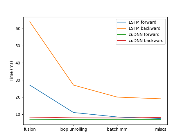
There are a number of additional optimizations that we did not cover in this post. In addition to the ones laid out in this post, we now see that our custom LSTM forward pass is on par with cuDNN. We are also working on optimizing backward more and expect to see improvements in future releases. Besides the speed that TorchScript provides, we introduced a much more flexible API that enable you to hand draft a lot more custom RNNs, which cuDNN could not provide.