A few weeks ago, TorchVision v0.11 was released packed with numerous new primitives, models and training recipe improvements which allowed achieving state-of-the-art (SOTA) results. The project was dubbed “TorchVision with Batteries Included” and aimed to modernize our library. We wanted to enable researchers to reproduce papers and conduct research more easily by using common building blocks. Moreover, we aspired to provide the necessary tools to Applied ML practitioners to train their models on their own data using the same SOTA techniques as in research. Finally, we wanted to refresh our pre-trained weights and offer better off-the-shelf models to our users, hoping that they would build better applications.
Though there is still much work to be done, we wanted to share with you some exciting results from the above work. We will showcase how one can use the new tools included in TorchVision to achieve state-of-the-art results on a highly competitive and well-studied architecture such as ResNet50 [1]. We will share the exact recipe used to improve our baseline by over 4.7 accuracy points to reach a final top-1 accuracy of 80.9% and share the journey for deriving the new training process. Moreover, we will show that this recipe generalizes well to other model variants and families. We hope that the above will influence future research for developing stronger generalizable training methodologies and will inspire the community to adopt and contribute to our efforts.
The Results
Using our new training recipe found on ResNet50, we’ve refreshed the pre-trained weights of the following models:
| Model | Accuracy@1 | Accuracy@5 |
|---|---|---|
| ResNet50 | 80.858 | 95.434 |
| ResNet101 | 81.886 | 95.780 |
| ResNet152 | 82.284 | 96.002 |
| ResNeXt50-32x4d | 81.198 | 95.340 |
Note that the accuracy of all models except RetNet50 can be further improved by adjusting their training parameters slightly, but our focus was to have a single robust recipe which performs well for all.
UPDATE: We have refreshed the majority of popular classification models of TorchVision, you can find the details on this blog post.
There are currently two ways to use the latest weights of the model.
Using the Multi-pretrained weight API
We are currently working on a new prototype mechanism which will extend the model builder methods of TorchVision to support multiple weights. Along with the weights, we store useful meta-data (such as the labels, the accuracy, links to recipe etc) and the preprocessing transforms necessary for using the models. Example:
  from PIL import Image
  from torchvision import prototype as P
  img = Image.open("test/assets/encode_jpeg/grace_hopper_517x606.jpg")

  # Initialize model
  weights = P.models.ResNet50_Weights.IMAGENET1K_V2
  model = P.models.resnet50(weights=weights)
  model.eval()

  # Initialize inference transforms
  preprocess = weights.transforms()

  # Apply inference preprocessing transforms
  batch = preprocess(img).unsqueeze(0)
  prediction = model(batch).squeeze(0).softmax(0)

  # Make predictions
  label = prediction.argmax().item()
  score = prediction[label].item()

  # Use meta to get the labels
  category_name = weights.meta['categories'][label]
  print(f"{category_name}: {100 * score}%")
Using the legacy API
Those who don’t want to use a prototype API have the option of accessing the new weights via the legacy API using the following approach:
  from torchvision.models import resnet

  # Overwrite the URL of the previous weights
  resnet.model_urls["resnet50"] = "https://download.pytorch.org/models/resnet50-11ad3fa6.pth"

  # Initialize the model using the legacy API
  model = resnet.resnet50(pretrained=True)

  # TODO: Apply preprocessing + call the model
  # ...
The Training Recipe
Our goal was to use the newly introduced primitives of TorchVision to derive a new strong training recipe which achieves state-of-the-art results for the vanilla ResNet50 architecture when trained from scratch on ImageNet with no additional external data. Though by using architecture specific tricks [2] one could further improve the accuracy, we’ve decided not to include them so that the recipe can be used in other architectures. Our recipe heavily focuses on simplicity and builds upon work by FAIR [3], [4], [5], [6], [7]. Our findings align with the parallel study of Wightman et al. [7], who also report major accuracy improvements by focusing on the training recipes.
Without further ado, here are the main parameters of our recipe:
  # Optimizer & LR scheme
  ngpus=8,
  batch_size=128,  # per GPU

  epochs=600,
  opt='sgd',
  momentum=0.9,

  lr=0.5,
  lr_scheduler='cosineannealinglr',
  lr_warmup_epochs=5,
  lr_warmup_method='linear',
  lr_warmup_decay=0.01,


  # Regularization and Augmentation
  weight_decay=2e-05,
  norm_weight_decay=0.0,

  label_smoothing=0.1,
  mixup_alpha=0.2,
  cutmix_alpha=1.0,
  auto_augment='ta_wide',
  random_erase=0.1,

  ra_sampler=True,
  ra_reps=4,


  # EMA configuration
  model_ema=True,
  model_ema_steps=32,
  model_ema_decay=0.99998,


  # Resizing
  interpolation='bilinear',
  val_resize_size=232,
  val_crop_size=224,
  train_crop_size=176,
Using our standard training reference script, we can train a ResNet50 using the following command:
torchrun --nproc_per_node=8 train.py --model resnet50 --batch-size 128 --lr 0.5 \
--lr-scheduler cosineannealinglr --lr-warmup-epochs 5 --lr-warmup-method linear \
--auto-augment ta_wide --epochs 600 --random-erase 0.1 --weight-decay 0.00002 \
--norm-weight-decay 0.0 --label-smoothing 0.1 --mixup-alpha 0.2 --cutmix-alpha 1.0 \
--train-crop-size 176 --model-ema --val-resize-size 232 --ra-sampler --ra-reps 4
Methodology
There are a few principles we kept in mind during our explorations:
- Training is a stochastic process and the validation metric we try to optimize is a random variable. This is due to the random weight initialization scheme employed and the existence of random effects during the training process. This means that we can’t do a single run to assess the effect of a recipe change. The standard practice is doing multiple runs (usually 3 to 5) and studying the summarization stats (such as mean, std, median, max, etc).
- There is usually a significant interaction between different parameters, especially for techniques that focus on Regularization and reducing overfitting. Thus changing the value of one can have effects on the optimal configurations of others. To account for that one can either adopt a greedy search approach (which often leads to suboptimal results but tractable experiments) or apply grid search (which leads to better results but is computationally expensive). In this work, we used a mixture of both.
- Techniques that are non-deterministic or introduce noise usually require longer training cycles to improve model performance. To keep things tractable, we initially used short training cycles (small number of epochs) to decide which paths can be eliminated early and which should be explored using longer training.
- There is a risk of overfitting the validation dataset [8] because of the repeated experiments. To mitigate some of the risk, we apply only training optimizations that provide a significant accuracy improvements and use K-fold cross validation to verify optimizations done on the validation set. Moreover we confirm that our recipe ingredients generalize well on other models for which we didn’t optimize the hyper-parameters.
Break down of key accuracy improvements
As discussed in earlier blogposts, training models is not a journey of monotonically increasing accuracies and the process involves a lot of backtracking. To quantify the effect of each optimization, below we attempt to show-case an idealized linear journey of deriving the final recipe starting from the original recipe of TorchVision. We would like to clarify that this is an oversimplification of the actual path we followed and thus it should be taken with a grain of salt.
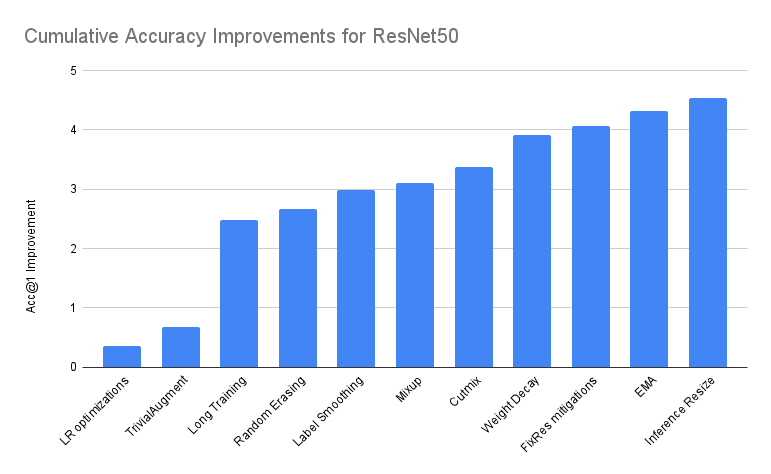
In the table below, we provide a summary of the performance of stacked incremental improvements on top of Baseline. Unless denoted otherwise, we report the model with best Acc@1 out of 3 runs:
| Accuracy@1 | Accuracy@5 | Incremental Diff | Absolute Diff | |
|---|---|---|---|---|
| ResNet50 Baseline | 76.130 | 92.862 | 0.000 | 0.000 |
| + LR optimizations | 76.494 | 93.198 | 0.364 | 0.364 |
| + TrivialAugment | 76.806 | 93.272 | 0.312 | 0.676 |
| + Long Training | 78.606 | 94.052 | 1.800 | 2.476 |
| + Random Erasing | 78.796 | 94.094 | 0.190 | 2.666 |
| + Label Smoothing | 79.114 | 94.374 | 0.318 | 2.984 |
| + Mixup | 79.232 | 94.536 | 0.118 | 3.102 |
| + Cutmix | 79.510 | 94.642 | 0.278 | 3.380 |
| + Weight Decay tuning | 80.036 | 94.746 | 0.526 | 3.906 |
| + FixRes mitigations | 80.196 | 94.672 | 0.160 | 4.066 |
| + EMA | 80.450 | 94.908 | 0.254 | 4.320 |
| + Inference Resize tuning * | 80.674 | 95.166 | 0.224 | 4.544 |
| + Repeated Augmentation ** | 80.858 | 95.434 | 0.184 | 4.728 |
*The tuning of the inference size was done on top of the last model. See below for details.
** Community contribution done after the release of the article. See below for details.
Baseline
Our baseline is the previously released ResNet50 model of TorchVision. It was trained with the following recipe:
  # Optimizer & LR scheme
  ngpus=8,
  batch_size=32,  # per GPU

  epochs=90,
  opt='sgd',
  momentum=0.9,

  lr=0.1,
  lr_scheduler='steplr',
  lr_step_size=30,
  lr_gamma=0.1,


  # Regularization
  weight_decay=1e-4,


  # Resizing
  interpolation='bilinear',
  val_resize_size=256,
  val_crop_size=224,
  train_crop_size=224,
Most of the above parameters are the defaults on our training scripts. We will start building on top of this baseline by introducing optimizations until we gradually arrive at the final recipe.
LR optimizations
There are a few parameter updates we can apply to improve both the accuracy and the speed of our training. This can be achieved by increasing the batch size and tuning the LR. Another common method is to apply warmup and gradually increase our learning rate. This is beneficial especially when we use very high learning rates and helps with the stability of the training in the early epochs. Finally, another optimization is to apply Cosine Schedule to adjust our LR during the epochs. A big advantage of cosine is that there are no hyper-parameters to optimize, which cuts down our search space.
Here are the additional optimizations applied on top of the baseline recipe. Note that we’ve run multiple experiments to determine the optimal configuration of the parameters:
  batch_size=128,  # per GPU

  lr=0.5,
  lr_scheduler='cosineannealinglr',
  lr_warmup_epochs=5,
  lr_warmup_method='linear',
  lr_warmup_decay=0.01,
The above optimizations increase our top-1 Accuracy by 0.364 points comparing to the baseline. Note that in order to combine the different LR strategies we use the newly introduced SequentialLR scheduler.
TrivialAugment
The original model was trained using basic augmentation transforms such as Random resized crops and horizontal flips. An easy way to improve our accuracy is to apply more complex “Automatic-Augmentation” techniques. The one that performed best for us is TrivialAugment [9], which is extremely simple and can be considered “parameter free”, which means it can help us cut down our search space further.
Here is the update applied on top of the previous step:
auto_augment='ta_wide',
The use of TrivialAugment increased our top-1 Accuracy by 0.312 points compared to the previous step.
Long Training
Longer training cycles are beneficial when our recipe contains ingredients that behave randomly. More specifically as we start adding more and more techniques that introduce noise, increasing the number of epochs becomes crucial. Note that at early stages of our exploration, we used relatively short cycles of roughly 200 epochs which was later increased to 400 as we started narrowing down most of the parameters and finally increased to 600 epochs at the final versions of the recipe.
Below we see the update applied on top of the earlier steps:
epochs=600,
This further increases our top-1 Accuracy by 1.8 points on top of the previous step. This is the biggest increase we will observe in this iterative process. It’s worth noting that the effect of this single optimization is overstated and somehow misleading. Just increasing the number of epochs on top of the old baseline won’t yield such significant improvements. Nevertheless the combination of the LR optimizations with strong Augmentation strategies helps the model benefit from longer cycles. It’s also worth mentioning that the reason we introduce the lengthy training cycles so early in the process is because in the next steps we will introduce techniques that require significantly more epochs to provide good results.
Random Erasing
Another data augmentation technique known to help the classification accuracy is Random Erasing [10], [11]. Often paired with Automatic Augmentation methods, it usually yields additional improvements in accuracy due to its regularization effect. In our experiments we tuned only the probability of applying the method via a grid search and found that it’s beneficial to keep its probability at low levels, typically around 10%.
Here is the extra parameter introduced on top of the previous:
random_erase=0.1,
Applying Random Erasing increases our Acc@1 by further 0.190 points.
Label Smoothing
A good technique to reduce overfitting is to stop the model from becoming overconfident. This can be achieved by softening the ground truth using Label Smoothing [12]. There is a single parameter which controls the degree of smoothing (the higher the stronger) that we need to specify. Though optimizing it via grid search is possible, we found that values around 0.05-0.15 yield similar results, so to avoid overfitting it we used the same value as on the paper that introduced it.
Below we can find the extra config added on this step:
label_smoothing=0.1,
We use PyTorch’s newly introduced CrossEntropyLoss label_smoothing parameter and that increases our accuracy by an additional 0.318 points.
Mixup and Cutmix
Two data augmentation techniques often used to produce SOTA results are Mixup and Cutmix [13], [14]. They both provide strong regularization effects by softening not only the labels but also the images. In our setup we found it beneficial to apply one of them randomly with equal probability. Each is parameterized with a hyperparameter alpha, which controls the shape of the Beta distribution from which the smoothing probability is sampled. We did a very limited grid search, focusing primarily on common values proposed on the papers.
Below you will find the optimal values for the alpha parameters of the two techniques:
mixup_alpha=0.2,
cutmix_alpha=1.0,
Applying mixup increases our accuracy by 0.118 points and combining it with cutmix improves it by additional 0.278 points.
Weight Decay tuning
Our standard recipe uses L2 regularization to reduce overfitting. The Weight Decay parameter controls the degree of the regularization (the larger the stronger) and is applied universally to all learned parameters of the model by default. In this recipe, we apply two optimizations to the standard approach. First we perform grid search to tune the parameter of weight decay and second we disable weight decay for the parameters of the normalization layers.
Below you can find the optimal configuration of weight decay for our recipe:
weight_decay=2e-05,
norm_weight_decay=0.0,
The above update improves our accuracy by a further 0.526 points, providing additional experimental evidence for a known fact that tuning weight decay has significant effects on the performance of the model. Our approach for separating the Normalization parameters from the rest was inspired by ClassyVision’s approach.
FixRes mitigations
An important property identified early in our experiments is the fact that the models performed significantly better if the resolution used during validation was increased from the 224×224 of training. This effect is studied in detail on the FixRes paper [5] and two mitigations are proposed: a) one could try to reduce the training resolution so that the accuracy on the validation resolution is maximized or b) one could fine-tune the model on a two-phase training so that it adjusts on the target resolution. Since we didn’t want to introduce a 2-phase training, we went for option a). This means that we reduced the train crop size from 224 and used grid search to find the one that maximizes the validation on resolution of 224×224.
Below you can see the optimal value used on our recipe:
val_crop_size=224,
train_crop_size=176,
The above optimization improved our accuracy by an additional 0.160 points and sped up our training by 10%.
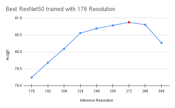
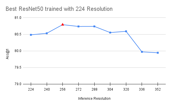
It’s worth noting that the FixRes effect still persists, meaning that the model continues to perform better on validation when we increase the resolution. Moreover, further reducing the training crop-size actually hurts the accuracy. This intuitively makes sense because one can only reduce the resolution so much before critical details start disappearing from the picture. Finally, we should note that the above FixRes mitigation seems to benefit models with similar depth to ResNet50. Deeper variants with larger receptive fields seem to be slightly negatively affected (typically by 0.1-0.2 points). Hence we consider this part of the recipe optional. Below we visualize the performance of the best available checkpoints (with the full recipe) for models trained with 176 and 224 resolution:
Exponential Moving Average (EMA)
EMA is a technique that allows one to push the accuracy of a model without increasing its complexity or inference time. It performs an exponential moving average on the model weights and this leads to increased accuracy and more stable models. The averaging happens every few iterations and its decay parameter was tuned via grid search.
Below you can see the optimal values for our recipe:
model_ema=True,
model_ema_steps=32,
model_ema_decay=0.99998,
The use of EMA increases our accuracy by 0.254 points comparing to the previous step. Note that TorchVision’s EMA implementation is build on top of PyTorch’s AveragedModel class with the key difference being that it averages not only the model parameters but also its buffers. Moreover, we have adopted tricks from Pycls which allow us to parameterize the decay in a way that doesn’t depend on the number of epochs.
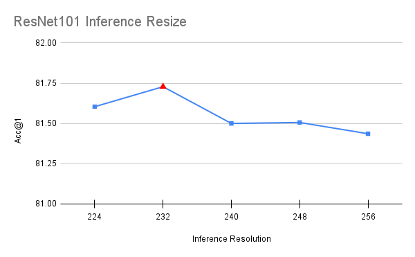
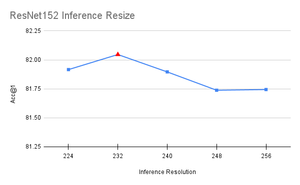
Inference Resize tuning
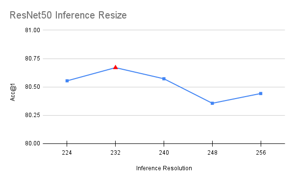
Unlike all other steps of the process which involved training models with different parameters, this optimization was done on top of the final model. During inference, the image is resized to a specific resolution and then a central 224×224 crop is taken from it. The original recipe used a resize size of 256, which caused a similar discrepancy as the one described on the FixRes paper [5]. By bringing this resize value closer to the target inference resolution, one can improve the accuracy. To select the value we run a short grid search between interval [224, 256] with step of 8. To avoid overfitting, the value was selected using half of the validation set and confirmed using the other half.
Below you can see the optimal value used on our recipe:
val_resize_size=232,
The above is an optimization which improved our accuracy by 0.224 points. It’s worth noting that the optimal value for ResNet50 works also best for ResNet101, ResNet152 and ResNeXt50, which hints that it generalizes across models:
[UPDATE] Repeated Augmentation
Repeated Augmentation [15], [16] is another technique which can improve the overall accuracy and has been used by other strong recipes such as those at [6], [7]. Tal Ben-Nun, a community contributor, has further improved upon our original recipe by proposing training the model with 4 repetitions. His contribution came after the release of this article.
Below you can see the optimal value used on our recipe:
ra_sampler=True,
ra_reps=4,
The above is the final optimization which improved our accuracy by 0.184 points.
Optimizations that were tested but not adopted
During the early stages of our research, we experimented with additional techniques, configurations and optimizations. Since our target was to keep our recipe as simple as possible, we decided not to include anything that didn’t provide a significant improvement. Here are a few approaches that we took but didn’t make it to our final recipe:
- Optimizers: Using more complex optimizers such as Adam, RMSProp or SGD with Nesterov momentum didn’t provide significantly better results than vanilla SGD with momentum.
- LR Schedulers: We tried different LR Scheduler schemes such as StepLR and Exponential. Though the latter tends to work better with EMA, it often requires additional hyper-parameters such as defining the minimum LR to work well. Instead, we just use cosine annealing decaying the LR up to zero and choose the checkpoint with the highest accuracy.
- Automatic Augmentations: We’ve tried different augmentation strategies such as AutoAugment and RandAugment. None of these outperformed the simpler parameter-free TrivialAugment.
- Interpolation: Using bicubic or nearest interpolation didn’t provide significantly better results than bilinear.
- Normalization layers: Using Sync Batch Norm didn’t yield significantly better results than using the regular Batch Norm.
Acknowledgements
We would like to thank Piotr Dollar, Mannat Singh and Hugo Touvron for providing their insights and feedback during the development of the recipe and for their previous research work on which our recipe is based on. Their support was invaluable for achieving the above result. Moreover, we would like to thank Prabhat Roy, Kai Zhang, Yiwen Song, Joel Schlosser, Ilqar Ramazanli, Francisco Massa, Mannat Singh, Xiaoliang Dai, Samuel Gabriel, Allen Goodman and Tal Ben-Nun for their contributions to the Batteries Included project.
References
- Kaiming He, Xiangyu Zhang, Shaoqing Ren, Jian Sun. “Deep Residual Learning for Image Recognition”.
- Tong He, Zhi Zhang, Hang Zhang, Zhongyue Zhang, Junyuan Xie, Mu Li. “Bag of Tricks for Image Classification with Convolutional Neural Networks”
- Piotr Dollár, Mannat Singh, Ross Girshick. “Fast and Accurate Model Scaling”
- Tete Xiao, Mannat Singh, Eric Mintun, Trevor Darrell, Piotr Dollár, Ross Girshick. “Early Convolutions Help Transformers See Better”
- Hugo Touvron, Andrea Vedaldi, Matthijs Douze, Hervé Jégou. “Fixing the train-test resolution discrepancy
- Hugo Touvron, Matthieu Cord, Matthijs Douze, Francisco Massa, Alexandre Sablayrolles, Hervé Jégou. “Training data-efficient image transformers & distillation through attention”
- Ross Wightman, Hugo Touvron, Hervé Jégou. “ResNet strikes back: An improved training procedure in timm”
- Benjamin Recht, Rebecca Roelofs, Ludwig Schmidt, Vaishaal Shankar. “Do ImageNet Classifiers Generalize to ImageNet?”
- Samuel G. Müller, Frank Hutter. “TrivialAugment: Tuning-free Yet State-of-the-Art Data Augmentation”
- Zhun Zhong, Liang Zheng, Guoliang Kang, Shaozi Li, Yi Yang. “Random Erasing Data Augmentation”
- Terrance DeVries, Graham W. Taylor. “Improved Regularization of Convolutional Neural Networks with Cutout”
- Christian Szegedy, Vincent Vanhoucke, Sergey Ioffe, Jon Shlens, Zbigniew Wojna. “Rethinking the Inception Architecture for Computer Vision”
- Hongyi Zhang, Moustapha Cisse, Yann N. Dauphin, David Lopez-Paz. “mixup: Beyond Empirical Risk Minimization”
- Sangdoo Yun, Dongyoon Han, Seong Joon Oh, Sanghyuk Chun, Junsuk Choe, Youngjoon Yoo. “CutMix: Regularization Strategy to Train Strong Classifiers with Localizable Features”
- Elad Hoffer, Tal Ben-Nun, Itay Hubara, Niv Giladi, Torsten Hoefler, Daniel Soudry. “Augment your batch: better training with larger batches”
- Maxim Berman, Hervé Jégou, Andrea Vedaldi, Iasonas Kokkinos, Matthijs Douze. “Multigrain: a unified image embedding for classes and instances”