Diffusion models for image and video generation have been surging in popularity, delivering super-realistic visual media. However, their adoption is often constrained by the sheer requirements in memory and compute. Quantization is essential for efficient serving of these models.
In this post, we demonstrate reproducible end-to-end inference speedups of up to 1.26x with MXFP8 and 1.68x with NVFP4 with diffusers and torchao on the Flux.1-Dev, QwenImage, and LTX-2 models on NVIDIA B200. We also outline how we used selective quantization, CUDA Graphs, and LPIPS as a measure to iterate on the accuracy and optimal performance of these models. The code to reproduce the experiments in this post is here.
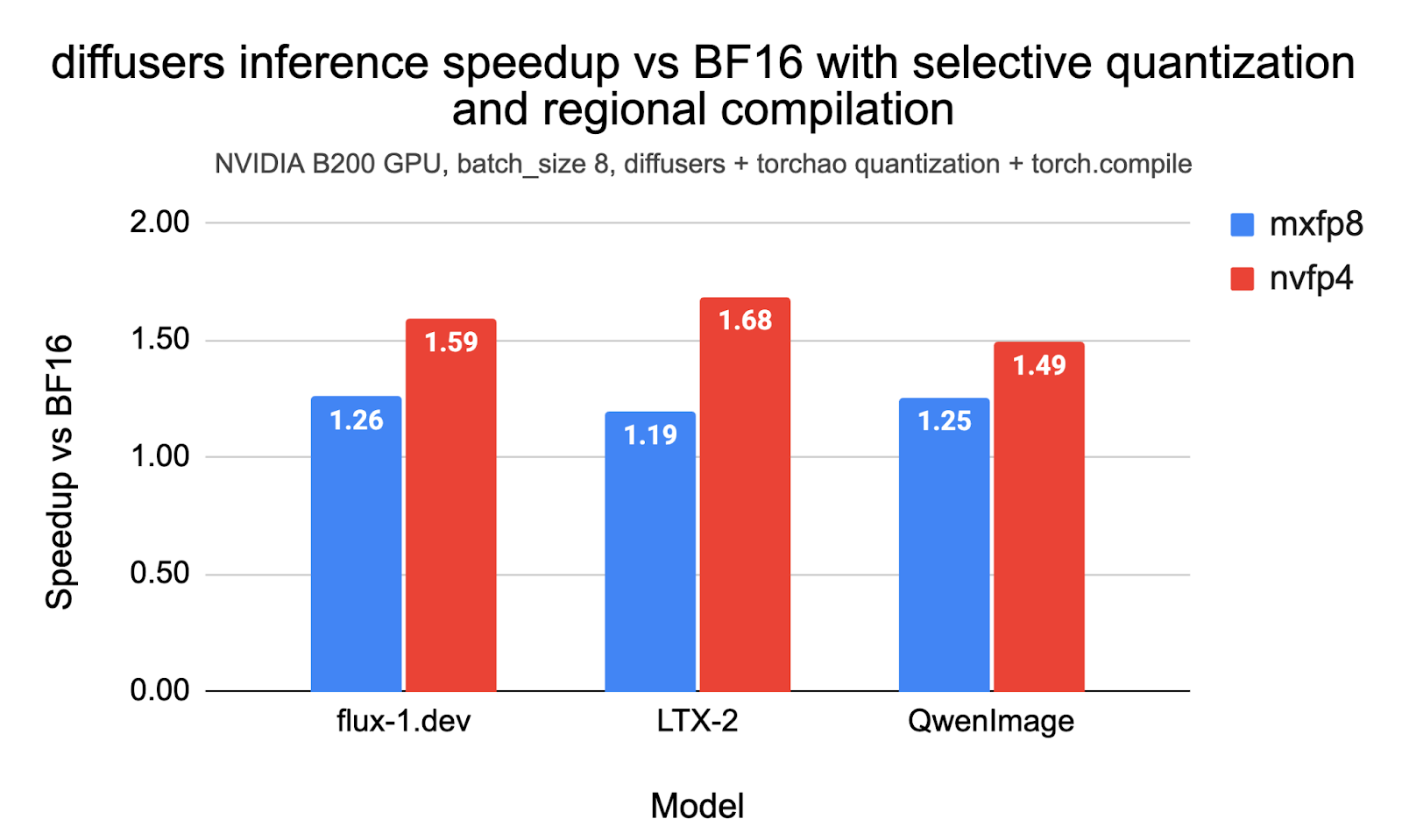 Table of contents:
- Background on MXPF8 and NVFP4
- Basic Usage with Diffusers and TorchAO
- Benchmark Results
- Technical Considerations
Background on MXFP8 and NVFP4
MXFP8 and NVFP4 are microscaling formats supported natively by NVIDIA’s Blackwell architecture (e.g., B200 GPUs). Unlike standard quantization, which scales an entire tensor, microscaling groups elements into small blocks (e.g., 16 or 32 values) that share a high-precision scale factor. This allows for significantly lower bit-depths while preserving dynamic range and accuracy.
- MXFP8 (OCP Microscaling FP8): An 8-bit industry-standard format (E4M3/E5M2) from the Open Compute Project (OCP). It uses a block size of 32 with 8-bit scaling. It provides a “sweet spot” balance, delivering faster inference than BF16 with virtually no loss in visual quality (lower LPIPS), and often achieves the lowest latency at smaller batch sizes.
- NVFP4 (NVIDIA FP4): A 4-bit floating-point format (E2M1) uniquely accelerated by Blackwell Tensor Cores. It uses a block size of 16 with FP8 scaling factors. It offers the highest theoretical throughput and lowest memory footprint (approx. 3.5x smaller than BF16), making it ideal for high-batch, compute-bound workloads.
Refer to this post to know more.
Basic Usage with diffusers and TorchAO
Prerequisites
NVFP4 requires a CUDA capability of at least 10.0. So, make sure you have a GPU that fits the bill. The benchmarks presented in this document were conducted on a B200 machine (B200 DGX).
For the virtual environment, you can use conda:
conda create -n nvfp4 python=3.11 -y

conda activate nvfp4

pip install --pre torch --index-url
https://download.pytorch.org/whl/nightly/cu130

pip install --pre torchao --index-url
https://download.pytorch.org/whl/nightly/cu130

pip install --pre mslk --index-url
https://download.pytorch.org/whl/nightly/cu130

pip install diffusers transformers accelerate sentencepiece protobuf av imageio-ffmpeg
At the time of writing, the nightlies were 2.12.0.dev20260315+cu130, 0.17.0.dev20260316+cu130, and 2026.3.15+cu130 for PyTorch, TorchAO, and MSLK, respectively.
Some models require users to be authenticated on the Hugging Face Hub platform. So, please make sure to run hf auth login before running the examples, if not already done.
Basic Usage
Using the NVFP4 quantization config from TorchAO is straightforward with its native integration in Diffusers:
from diffusers import DiffusionPipeline, TorchAoConfig, PipelineQuantizationConfig

import torch

from torchao.prototype.mx_formats.inference_workflow import (
    NVFP4DynamicActivationNVFP4WeightConfig,
)

config = NVFP4DynamicActivationNVFP4WeightConfig(
    use_dynamic_per_tensor_scale=True, use_triton_kernel=True,
)
pipe_quant_config = PipelineQuantizationConfig(
    quant_mapping={"transformer": TorchAoConfig(config)}
)

pipe = DiffusionPipeline.from_pretrained(
    "black-forest-labs/FLUX.1-dev",
    torch_dtype=torch.bfloat16,
    quantization_config=pipe_quant_config
).to("cuda")
pipe.transformer.compile_repeated_blocks(fullgraph=True)

pipe_call_kwargs = {
    "prompt": "A cat holding a sign that says hello world",
    "height": 1024,
    "width": 1024,
    "guidance_scale": 3.5,
    "num_inference_steps": 28,
    "max_sequence_length": 512,
    "num_images_per_prompt": 1,
    "generator": torch.manual_seed(0),
}
result = pipe(**pipe_call_kwargs)
image = result.images[0]
image.save("my_image.png")
The code snippet above quantizes every torch.nn.Linear layer of the model.
For this post, we always use regional compilation with fullgraph=True, as it significantly reduces compilation time and yields results almost as good as full model compilation. Know more about regional compilation from here.
Recipe Selection
The code snippet below shows how to configure MXFP8 and NVFP4 inference with TorchAO:
# MXFP8

quant_config = MXDynamicActivationMXWeightConfig(
    activation_dtype=torch.float8_e4m3fn,
    weight_dtype=torch.float8_e4m3fn,
    kernel_preference=KernelPreference.AUTO,
)

# NVFP4

quant_config = NVFP4DynamicActivationNVFP4WeightConfig(
    use_dynamic_per_tensor_scale=True,
    use_triton_kernel=True,
)
Benchmark Results
Flux.1-Dev
The following inference params were used during benchmarking FLUX.1-dev:
{
    "prompt": "A cat holding a sign that says hello world",
    "height": 1024,
    "width": 1024,
    "guidance_scale": 3.5,
    "num_inference_steps": 28,
    "max_sequence_length": 512,
}
Performance and Peak Memory
First, we present latency and peak memory consumption across different settings and different benchmarks, with speedups up to 1.26x with MXFP8 and up to 1.59x with NVFP4. Note that these results use selective quantization, wherein we exclude certain layers from getting quantized. We discuss more about selective quantization later in this post.
Flux-1.dev performance and peak memory with MXFP8 and NVFP4 quantization |
||||
|---|---|---|---|---|
| Quant Mode | Batch Size | Latency (s) | Memory (GB) | Speedup vs BF16 |
| None | 1 | 2.10 | 38.34 | 1.00 |
| MXFP8 | 1 | 1.75 | 26.90 | 1.21 |
| NVFP4 | 1 | 1.41 | 21.33 | 1.50 |
| None | 4 | 7.87 | 44.39 | 1.00 |
| MXFP8 | 4 | 6.36 | 32.95 | 1.24 |
| NVFP4 | 4 | 5.09 | 27.39 | 1.55 |
| None | 8 | 15.57 | 53.00 | 1.00 |
| MXFP8 | 8 | 12.40 | 41.56 | 1.26 |
| NVFP4 | 8 | 9.81 | 36.00 | 1.59 |
NVIDIA B200, selective quantization, torch.compile with regional compilation; batch_size=1 uses torch.compile(..., mode='reduce-overhead'). Quant Mode “None” means no quantization.
Accuracy
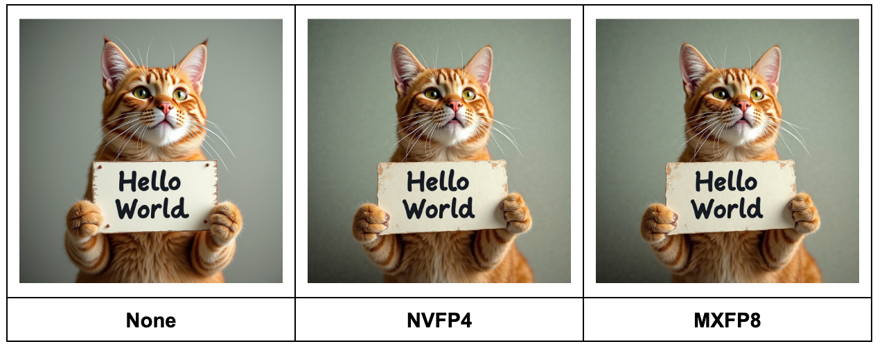
The MXFP8 and NVFP4 images generated for a test prompt are close to the bfloat16 baseline:
For a more thorough accuracy evaluation, we computed the mean LPIPS score between the bfloat16 images (baseline) and MXFP8|NVFP4 images (experiment), averaged over the prompts in the Drawbench dataset:
Flux-1.dev mean LPIPS score with MXFP8 and NVFP4 quantization |
|
|---|---|
| Quant Mode | Mean LPIPS on Drawbench |
| None | 0 |
| MXFP8 | 0.11 |
| NVFP4 | 0.44 |
NVIDIA B200, selective quantization, torch.compile with regional compilation.
An LPIPS score of zero means “identical images”, and lower LPIPS scores correspond to higher perceptual similarity. The code we used to compute the mean LPIPS score is here. Please see the LPIPS section further in this post for more details on accuracy evaluations with LPIPS.
LTX-2
For LTX-2, we enabled tiling on the VAE to keep the memory requirements manageable. The following inference-time parameters were used to obtain the results:
 {
        "prompt": (
              "INT. HOME OFFICE - DAY. Soft natural daylight lights a desk with an open laptop. The camera holds a steady medium shot. A small real house cat sits naturally on all fours in front of the laptop, much smaller than the desk and computer. The cat looks at the screen curiously. Suddenly, with a soft magical sparkle effect, a pair of tiny reading glasses appears in midair and gently lands on the cat's face. A faint whimsical chime sound plays. The cat pauses for a split second, then begins pressing the keyboard clumsily with one paw, producing rapid typing sounds. The laptop screen glow reflects softly on the cat's fur while light playful music continues."
        ),
        "negative_prompt": "worst quality, inconsistent motion, blurry, jittery, distorted",
        "width": 768,
        "height": 512,
        "num_frames": 121,
        "frame_rate": 24.0,
        "num_inference_steps": 40,
        "guidance_scale": 4.0,
}
Performance and Peak Memory
LTX-2 performance and peak memory with MXFP8 and NVFP4 quantization |
||||
|---|---|---|---|---|
| Quant Mode | Batch Size | Latency (s) | Memory (GB) | Speedup |
| None | 1 | 16.230 | 72.77 | 1.00 |
| MXFP8 | 1 | 13.724 | 54.54 | 1.18 |
| NVFP4 | 1 | 10.374 | 45.72 | 1.56 |
| None | 4 | 61.591 | 87.61 | 1.00 |
| MXFP8 | 4 | 50.956 | 69.38 | 1.21 |
| NVFP4 | 4 | 36.963 | 60.56 | 1.67 |
| None | 8 | 122.427 | 107.40 | 1.00 |
| MXFP8 | 8 | 102.546 | 89.18 | 1.19 |
| NVFP4 | 8 | 72.689 | 80.36 | 1.68 |
NVIDIA B200, selective quantization, torch.compile with regional compilation. Quant Mode “None” means no quantization.
Accuracy
Check out this link for a comparison of the video results on a test prompt. Calculating eval scores over a prompt dataset (like we did for Flux-1.dev) is left for a future study.
QwenImage
The following inference-time parameters were used to obtain the results:
 {
    "prompt": "A cat holding a sign that says hello world",
    "negative_prompt": " ",
    "height": 1024,
    "width": 1024,
    "true_cfg_scale": 4.0,
    "num_inference_steps": 50,
}
Performance and Peak Memory
QwenImage performance and peak memory with MXFP8 and NVFP4 quantization |
||||
|---|---|---|---|---|
| Quant Mode | Batch Size | Latency (s) | Memory (GB) | Speedup |
| None | 1 | 7.454 | 62.21 | 1.00 |
| MXFP8 | 1 | 6.430 | 55.65 | 1.16 |
| NVFP4 | 1 | 5.369 | 52.45 | 1.39 |
| None | 4 | 26.779 | 75.52 | 1.00 |
| MXFP8 | 4 | 21.835 | 68.97 | 1.23 |
| NVFP4 | 4 | 18.279 | 65.76 | 1.47 |
| None | 8 | 52.095 | 92.47 | 1.00 |
| MXFP8 | 8 | 41.569 | 85.91 | 1.25 |
| NVFP4 | 8 | 34.969 | 82.7 | 1.49 |
NVIDIA B200, selective quantization, torch.compile with regional compilation, batch_size=1 uses torch.compile(..., mode='reduce-overhead'). Quant Mode “None” means no quantization.
Accuracy
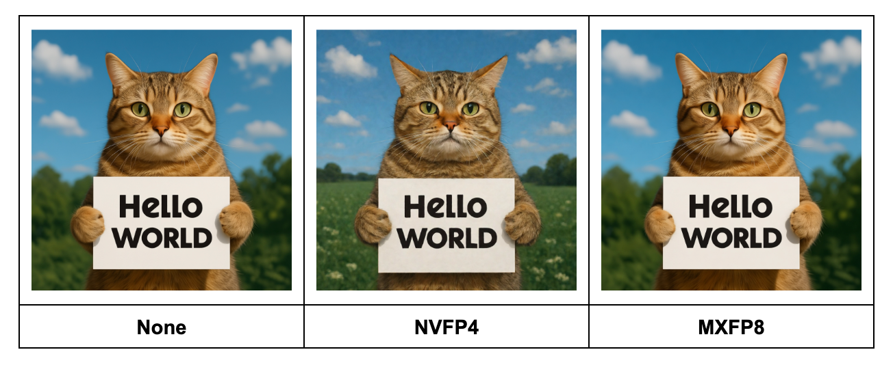
The MXFP8 and NVFP4 images generated for a test prompt are close to the bfloat16 baseline, with NVFP4 showing slightly larger differences vs MXFP8:
In the following table, we report the LPIPS scores similar to Flux.1-Dev.
QwenImage mean LPIPS score with MXFP8 and NVFP4 quantization |
|
|---|---|
| Quant Mode | Mean LPIPS on Drawbench |
| None | 0 |
| MXFP8 | 0.34 |
| NVFP4 | 0.41 |
Note: In our experiments, we found QwenImage to be more sensitive to quantization than Flux.1-Dev, as evidenced by the higher mean MXFP8 LPIPS score of 0.34 for QwenImage (compared to a mean LPIPS score of 0.11 for MXP8 on Flux-1.Dev). Reducing the mean LPIPS score for QwenImage further via more aggressive selective quantization or more advanced numerical algorithms (GPTQ, QAT, etc) is left for a future study.
Technical Considerations
In this section, we share how we used selective quantization, CUDA Graphs, and LPIPS to iterate on the performance and accuracy metrics presented in this post.
Optimizing Accuracy and Performance with Selective Quantization
We used selective quantization to optimize for latency (all models) and LPIPS (Flux-1.dev), skipping layers based on two simple heuristics:
- If the weight or activation shape of a
torch.nn.Linearis too small to benefit from quantizationmin(M, K, N) < 1024), skip it. This is to ensure that the speedup from quantizing the matrix multiply is larger than the additional overhead of quantizing the activation (more context: here).- A tutorial for how to find the weight and activation shapes in your model using
torchaotooling is here. Note that even if the weight is large, a small activation shape could make quantization not profitable.
- A tutorial for how to find the weight and activation shapes in your model using
- If the layer is likely to meaningfully contribute to model accuracy (such as embeddings, normalization), skip it.
- To apply this on your model, you can print out the model (
print(model)) and inspect the FQNs manually, then skip the FQNs you suspect could be impacting accuracy based on your knowledge of the model architecture.
- To apply this on your model, you can print out the model (
The exact heuristics we used for each model are:
To quantify the impact of selective quantization, we measure performance, memory, and mean LPIPS (with AlexNet) between the images with pure Bfloat16 and images generated with NVFP4 and MXFP8.
Impact of full vs selective quantization on Flux-1.dev |
|||
|---|---|---|---|
| Quant Mode | LPIPS | Latency (s) | Memory (GB) |
| MXFP8 + full quantization | 0.138128 | 1.774 | 26.84 |
| MXFP8 + selective quantization | 0.107562 | 1.746 | 26.90 |
| NVFP4 + full quantization | 0.479679 | 2.112 | 21.25 |
| NVFP4 + selective quantization | 0.438337 | 2.076 | 21.33 |
(Lower LPIPS is better, with LPIPS of ~0.1 usually meaning that the images are nearly indistinguishable. LPIPS computation code is available here).
As we can notice from the results above, excluding certain layers from quantization (aka “selective quantization”) provides the best trade-off between latency, peak memory consumption, and LPIPS. Therefore, we follow the recipe of selective quantization for the rest of the two models reported in this post.
We used simple heuristics to find our selective quantization recipes. There are more advanced approaches for selective quantization, such as this layer sensitivity study.
Note that while iterating on our selective quantization recipes, we found performance gaps in TorchAO’s kernel for quantizing tensors to NVFP4. We improved NVFP4 performance in this PR by upgrading the `to_nvfp4` kernel to use MSLK.
Improving CPU Overhead with CUDA Graphs
We noticed that when using NVFP4 with small batch sizes like 1, CPU overhead tends to have a nontrivial impact on latency improvements. To significantly reduce this overhead, we used the “reduce-overhead” compilation mode, which enables CUDA graphs. Below, we provide the profile traces before and after applying CUDA Graphs.
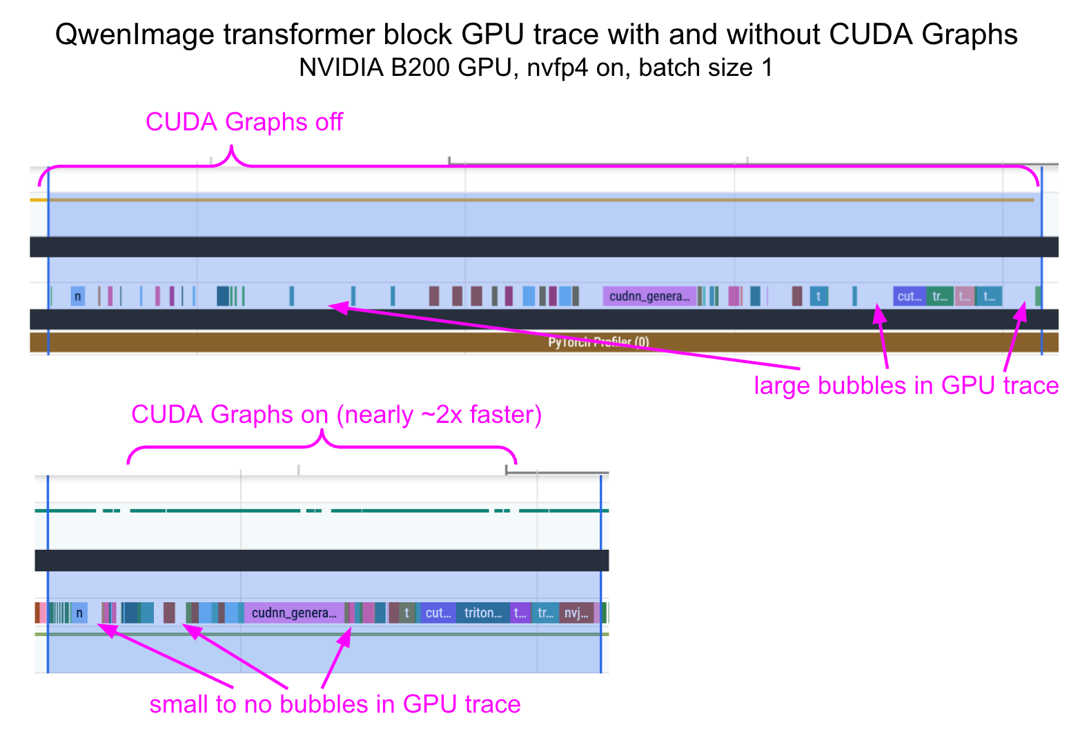
To cleanly compose torch.compile(..., mode='reduce-overhead') with the per-block compilation from the diffusers library, we had to wrap each transformer block in a function that clones its inputs. The PR to do this is here, showing a 1.81x speedup for QwenImage + nvfp4 at batch_size==1.
Evaluating Image Generation Accuracy with LPIPS
We used the LPIPS (GitHub) metric to compare how similar images generated by a quantized model are from the images generated by the baseline (bfloat16) model. In pseudocode:
lpips_scores = []

for text_prompt in dataset:
    generator = torch.Generator(device=device).manual_seed(seed)
    kwargs = {"prompt": prompt, "generator": generator, ...}
    image_baseline = pipe_bf16(**kwargs)
    image_quantized = pipe_quantized(**kwargs)
    lpips_score = calculate_lpips_score(image_baseline, image_quantized)
    lpips_scores.append(lpips_score)

lpips_mean = lpips_scores.sum() / len(lpips_scores)
The actual code we used is here.
Example LPIPS Scores for Pairs of Images
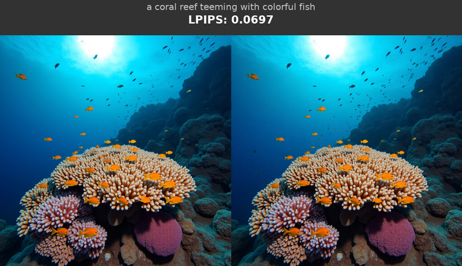
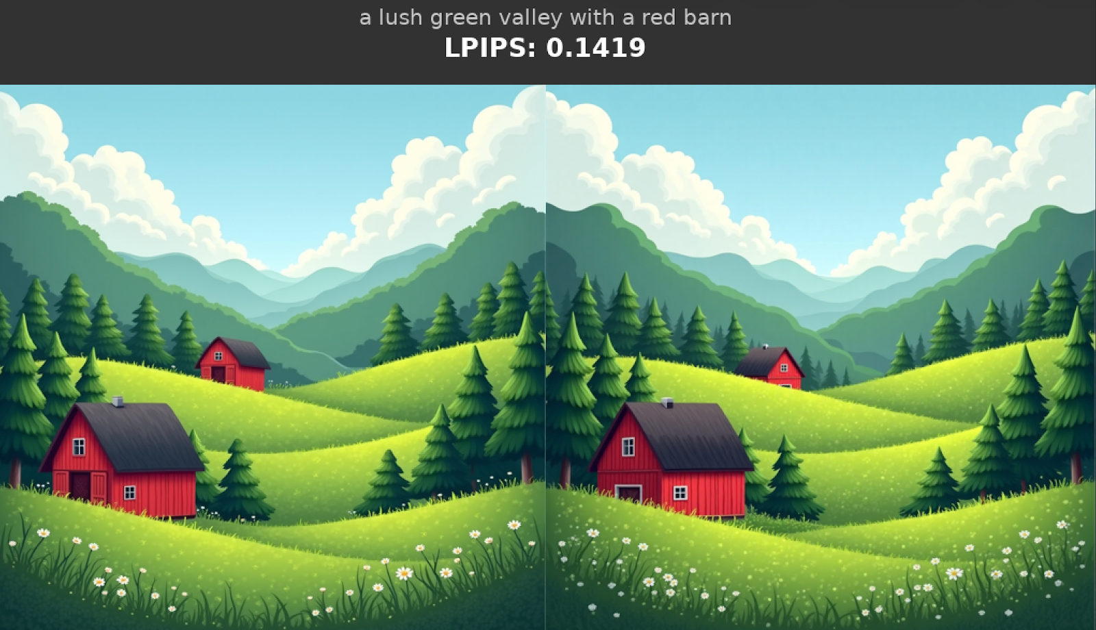
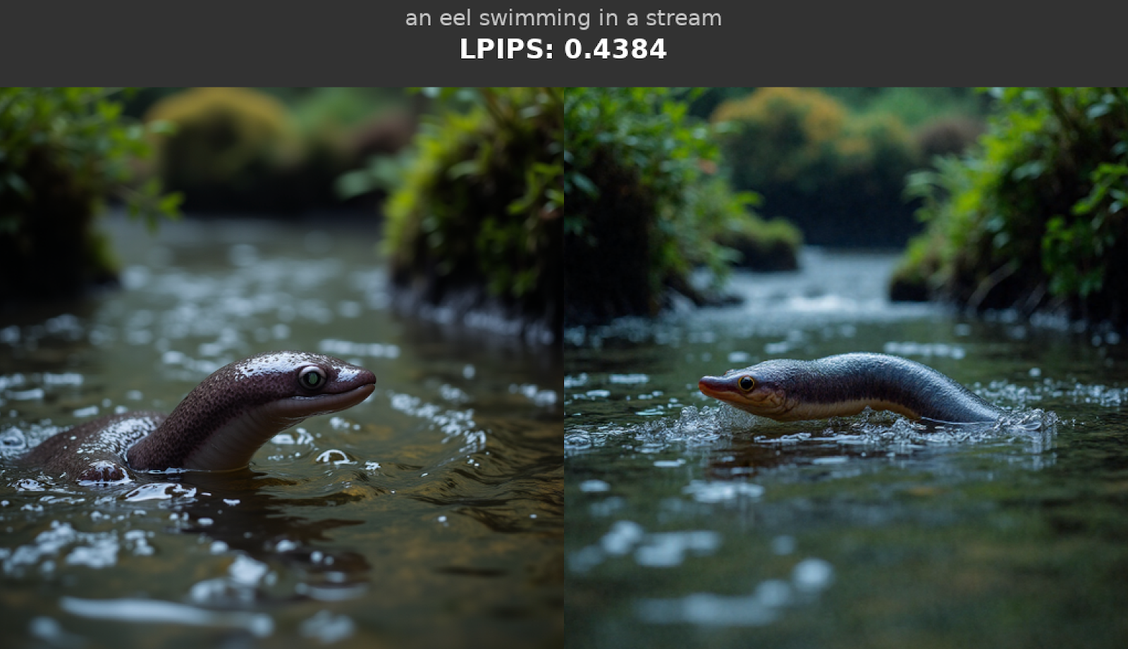
This section provides example LPIPS scores for pairs of images to help put the LPIPS metrics reported above into context, and enable readers to reason about “what is a good LPIPS score”.
The images below were generated with FLUX.1-dev. The images on the left are the baseline (bfloat16), and the images on the right are from quantizing every torch.nn.Linear of the model with MXFP8. The LPIPS scores are based on the comparison of the image on the right (experiment) to the image on the left (baseline).
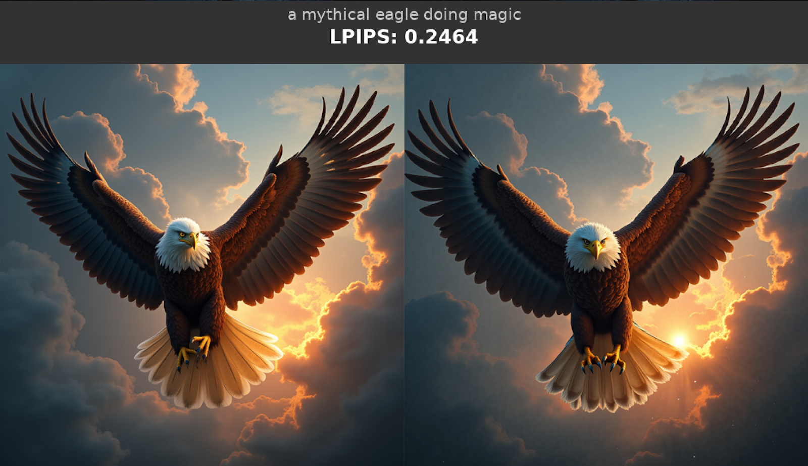
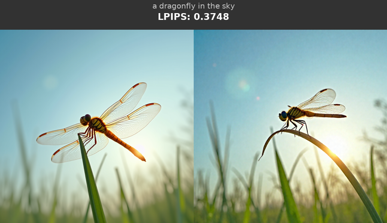
Below, we provide a similar comparison but with NVFP4 images on the right-hand side.
Conclusion
In this post, we investigated the performance of NVFP4 and MXFP8 quantization schemes on popular image and video generation models. We presented the recipes that provide a reasonable trade-off between speed, quality, and memory. We also uncovered some important issues that can get in the way of optimal performance and how we can approach them. We hope these recipes will help improve the performance of your image and video generation workloads.
Resources
- Code repository
- TorchAO docs:
- Diffusers x TorchAO integration
All outputs can be found here