
In this blog post, we explore the kernel design details presented in the paper Fast and Simplex: 2-Simplicial Attention in Triton [1]. We begin by modeling the 2-Simplicial attention algorithm with a hardware-aligned design, then completely rewrite the entire kernel in TLX (Triton Low-Level Extensions) [2] using modern GPU kernel techniques. Leveraging TLX, we achieve up to 588 Tensor Core BF16 TFLOPs, approximately 60% tensor core utilization, in the forward pass of 2-Simplicial attention on the NVIDIA H100 GPU, around 1.74x speedup of the original Triton kernel’s 337 peak TFLOPs.
Code Repository: https://github.com/pytorch/FBGEMM/tree/main/fbgemm_gpu/experimental/simplicial_attention
† Work done while at Meta
Recap of 2-Simplicial Attention
As large language models continue to scale, it becomes increasingly challenging to acquire sufficient high-quality training tokens. Enhancing the token efficiency of attention mechanisms is crucial in addressing this issue. One promising advancement is 2-Simplicial Attention (Algorithm 1), which uses trilinear functions to model interactions between a query and two sets of keys (K1, K2) and two sets of values (V1, V2), to model complex interactions among triples of tokens, rather than just pairs as in standard dot-product attention. As first proposed in the paper Logic and the 2-Simplicial Transformer [3], 2-Simplicial attention increases the TFLOPs of the attention while mostly preserving the original model size. According to scaling law experiments, the 2-Simplicial attention has shown significant improvements in token efficiency, particularly for reasoning tasks such as mathematics and logical problem solving.


Figure 1: Visualization of 2-simplicial attention with 2D sliding window. Each rectangle represents the interaction between one query (Q) and a pair of keys (K′ and K). Blue rectangles highlight specific query-key pair interactions within the sliding window structure.
2D Sliding Window Attention

Figure 2: Comparison Sliding Window Attention and 2-Simplicial Sliding Window Attention
Because full 2-simplicial attention grows cubically with sequence length O(N³), attending to an entire sequence is impractical. We mitigate this cost with a two-dimensional sliding-window (defined in Figure 2-b and shown in Figure 1) defined by two window sizes, W1 and W2. Each query token Q[i] only attends to
- the W1 nearest K1[i] / V1[i] pairs along the first dimension
- the W2 nearest K2[k] / V2[k] pairs along the second dimension
This locality constraint preserves the expressive power of 2-simplicial attention while keeping computation tractable.
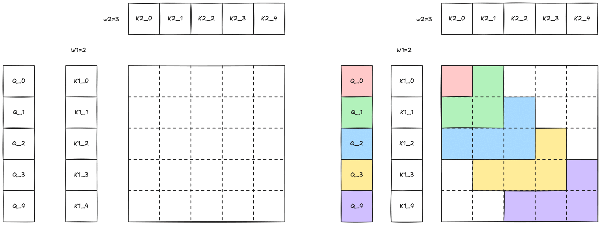
Figure 3: Illustration of 2-simplicial attention with 2D sliding window. The colored region, with the same color of the Q token, illustrates the two-dimensional neighborhood (W1 × W2) within which the query can attend to keys and values.
Introduction of TLX – Triton Low-Level Extensions
TLX (Triton Low-Level Extensions) is a language extension to the Triton DSL that combines high performance with developer productivity. It integrates seamlessly with Triton’s high-level Python API while adding warp-aware, hardware-close control over GPU kernel execution through a rich set of intrinsics. With native support for NVIDIA Hopper and Blackwell—and an extensible design for future architectures, including potential AMD GPUs—TLX enables shared memory tiling, register-backed accumulators, warp specialization, pipelined execution, and fine-grained warp-level synchronization.
Fast 2-Simplicial Attention – Hardware-Aligned Design
To make the kernel really efficient and achieve SOTA performance, we have a lot of hardware-aligned co-design between the model and the kernel. The proposed kernel design adopts the following key features.
Tensor Core Friendly
Since dot products are inherently binary operations between two tensors (dot_product), the presence of three tensors (trilinear_product) in 2-Simplicial Attention (detailed in Appendix [3]) presents a fundamental challenge: the computation CANNOT directly leverage Tensor Cores
To address this limitation, we develop a Tensor Core-compatible approach through strategic pre-computation. Our solution decomposes the Ternary operation into Binary components:
- First, we pre-compute the element-wise product of Q[i] and K1[s], equation (c) line-10, enabling Tensor Core computation for the subsequent multiplication with K2[t], equation (c) line-11
- Similarly, we pre-compute the element-wise product of V1[s] and V2[t], equation (c) line-13, allowing efficient Tensor Core computation of P with the combined V12[s][t], equation (c) line-14
This reformulation, shown in equation (c), transforms the 2-simplicial sliding window attention into a Tensor Core-friendly design and maintains the mathematical equivalence.

NOTE: ⊙ denotes element-wise multiplication
We considered two approaches for implementing the tensor core-friendly formulation as GPU kernels:
- Separate kernels: Implement pre-computation in one kernel, write results (Precomputed-QK1 and Precomputed-V1V2) to global memory (GMEM) and a custom dot-product attention kernel
- Fused kernel: Integrate the entire equation (c) into a single attention kernel
The first approach presents a significant drawback: substantially increased peak memory usage. Specifically, Precomputed-QK1 requires W1 times more memory than Q, and Precomputed-V1V2 requires (W1 + W2) times more memory than V. With typical values such as W1 = 32, W2 = 512, and N scaling with the model’s context window, the memory overhead becomes prohibitive for training models that incorporate 2-simplicial attention. Therefore, we adopted the second approach, implementing an end-to-end fused kernel for 2-simplicial sliding window attention.
Asymmetric Sliding Window
Asymmetric sliding window (W1 ≠ W2) versus symmetric sliding window (W1 = W2): experimental results [1] demonstrate that when W1 x W2 remains constant (maintaining identical Tensor Core TFLOPs), asymmetric configurations typically yield better model quality. For the hardware alignment, we employ small W1 and large W2 values (W1 = 32, W2 = 512 in our implementation) for the following reasons:
- Tensor Core friendly: Larger W2 values increase the Tensor Core to CUDA Core ratio, enhancing Tensor Core computation efficiency
- Persist all K1 and V1 tiles in Shared Memory (SMEM): According to Algorithm 2, each K1/V1 tile has shape [1, D] and requires W1 loads. With small W1, we can load all W1 K1/V1 tiles in SMEM with the shape [W1, D] per CTA outside loops, then reload individual [1, D] tiles from SMEM to registers during the W1-loop. For W1 = 32, D = 128, and BFloat16 precision, total size of K1 and V1 tiles is 16KB, approximately 7% of H100’s SMEM capacity.
Group Tiling of Heads – Pack GQA
In sliding window attention, each query Q token selects different sets of K tokens. When tiling along the sequence dimension, we must mask out certain QK pairs, resulting in wasted computation. This inefficiency is amplified in 2D sliding window attention. For example, with BLOCK_M = 64, BLOCK_KV = 128, N = 8192, W1 = 32, and W2 = 512, according to the calculation in Appendix [1]. Approximately 73.2% of computation is wasted.
Inspired by the Kernel Design of Native Sparse Attention [5], we pack all query heads of the same GQA KV head group into a single tile instead of tiling along the sequence dimension. This approach eliminates most 2D sliding window mask calculations. In our final implementation, sliding window masking is only required for the last W2-loop iteration in the first few CTAs, reducing the wasted ratio from 73.2% to 1.35% (details calculation in Appendix [1]).
Trade-off considerations: The drawback of head-dimension tiling is reduced flexibility in the configuration of the number of query heads. WGMMA [6] instructions require minimum M = 64. Configurations below 64 also waste computation. To balance mask efficiency and model flexibility, we can pack contiguous Q tokens with Q heads into a tile to meet the 64-size requirement (like PACK_GQA in FA3 decoding kernels). While the original paper uses GQA ratio 64, our implementation uses 128 to enable two consumer warp-group partitions across different Q tiles for the benchmark of peak TFLOPs.
V1 Tile Optimization
Consider the operation C = A @ B. WGMMA instructions allow matrix A storage in register memory (RMEM) or SMEM, while matrix B must reside in SMEM. Output tile C is stored in RMEM. For PV12 GEMM in attention, P (output of QK12 GEMM) resides in RMEM, and V2 (loaded via TMA) resides in SMEM. However, the broadcast multiplication operation for V1 and V2 equation (c), requires both operands in RMEM. This necessitates loading V2 from SMEM to RMEM, performing element-wise computation to generate V12, then storing V12 back to SMEM. This is an inefficient process.
We observed that PV GEMM output resides in RMEM, and since V1 is broadcast along the dot product dimension of PV12, it is mathematically equivalent to apply V1 to V2 before or after dot product with P.

Therefore, we optimized the algorithm to apply the V1 tile directly to PV GEMM output, eliminating redundant SMEM ↔ RMEM load/store operations.
NOTE: Why compute Q⊙K1 instead of K1⊙K2? It’s because
- K1⊙K2 can’t be pre-computed in the w1-loop. Pre-computing all combinations requires storing data of size w1 × w2 × D in SMEM, which is too large to hold
- The result of K1⊙K2 resides in RMEM, creating the same inefficiency we encounter with V1⊙V2

Figure 4: Illustration of Algorithm 2 Kernel Design
Based on all these features and the FlashAttention2 [3] algorithm, we conducted the fused 2-simplicial attention kernel algorithm – Algorithm 2. Compared to the dot-product attention, it introduces two nested inner loops for w1 and w2, with the innermost loop closely resembling the inner loop of FlashAttention2.

Algorithm 2 does more CUDA Core calculation, raising the question about whether CUDA Cores will become the performance bottleneck for the 2-Simplicial Attention kernel. Our analysis shows that CUDA Cores are not the limiting factor; detailed justification is provided in Appendix [5].
Adopting Modern GPU Techniques with TLX
Despite implementing all the optimizations mentioned above, our Triton kernel implementation remained significantly below state-of-the-art performance. Our best forward attention kernel can only achieve 34% Tensor Core utilization, while FlashAttention3 [4] has an impressive 75% utilization.
Analysis of the generated PTX code revealed that software pipelining and automatic warp specialization failed to work with the kernel. The software pipeline compiler backend couldn’t perform the necessary pattern matching and skipped optimization, while warp specialization triggered compilation errors specific to the 2-Simplicial attention implementation.
To rapidly integrate modern attention optimization techniques like FlashAttention3 [4] on Hopper architecture, including warp specialization, inter-warpgroup overlapping (pingpong scheduling), and intra-warpgroup overlapping (computation pipelining), we re-write the kernel using TLX. We developed three distinct versions:
- Kernel-1: Forward + Warp Specialization (described in Appendix [4] Algorithm 3)
- Kernel-2: Forward + Warp Specialization + Computation Pipelining
- Kernel-3: Forward + Warp Specialization + Pingpong Scheduling
NOTE: If you want to want to know more about Warp Specialization, Computation Pipelining, and Pingpong Scheduling on Hopper, please take a look at the paper – FlashAttention3 [4] and the Colfax Blog.

Figure 5 illustrates the idea of Kernel-3: Warp Specialization with Pingpong Scheduling, using two buffers in shared memory (SMEM) and two consumer groups. The producer (WarpGroup 0) begins by issuing TMA loads for two tiles of Q, one tile of K1, one tile of V1, and two tiles each of K2 and V2. The consumer warp groups wait for the corresponding tiles to arrive before performing their computations. Synchronization between the producer and consumers is managed via barriers.
Each consumer group operates on a different tile of Q but shares the same tiles of K1, V1, K2, and V2, while producing results for distinct output tiles. To maximize efficiency, pingpong scheduling ensures that only one warp group performs Tensor Core (WGMMA) operations at a time.
Figure 6 is the comparison of execution traces, captured with Proton [8], for Kernel-1 WS (top) and Kernel-3 WS with Pingpong scheduling (bottom). The traces highlight how Ping-Pong scheduling reduces Tensor Core bubbles within the inner w2-loop, leading to improved utilization of Tensor Core resources.

Figure 6: Illustration of Tensor Core Bubbles of Kernel-1 WS (top) and Kernel-3 WS + Pingpong (bottom)
Benchmark results show approximately neutral to 1% performance gain from Kernel-1 to Kernel-3. The modest gain likely reflects that, Kernel-1 already achieves partial overlap between GEMM and Softmax operations. Currently, Kernel-1 achieves 60% Tensor Core utilization, which is a significant improvement over the previous pure Triton implementation 34% Tensor Core utilization. Kernel-2 experiences performance regression due to register spilling issues. Theoretically, the combination of Warp Specialization, Computation Pipelining, and Pingpong Scheduling should yield the best performance.
Benchmarks
Based on the analysis in Appendix [5], Tensor Core TFLOPs significantly exceed CUDA Core TFLOPs. Therefore, for simplicity, we calculate only Tensor Core TFLOPs as our primary metric for kernel performance.
Please note the following behavior regarding 2D sliding window attention, here we assume W1 ≤ W2,
- When the total sequence length N < W1: The mechanism operates as 2D causal attention on both W1 and W2
- When W1 ≤ N < W2: The mechanism operates as a 1D sliding window on W1 and 1D causal attention on W2
- When N ≥ W2: The mechanism operates as a full 2D sliding window
For details on the Tensor Core TFLOPs calculation, please refer to Appendix [2].
The benchmark setup is detailed in [9]. We presented results in Figure 5 with the peak 588 TFLOPs.

Figure 7: Benchmark Result of Fast 2-Simplicial Attention Kernel – Fwd
NOTE: Small sequence lengths result in poor performance due to masked tiles. Specifically, for tokens where i < W2, a causal mask must be applied to the final tile to ensure j ≤ i. This reduces computational density of the final tiles for those tokens, along with adding cuda core overhead from masking computation. Conversely, for tokens where i ≥ W2 and W2 % BLOCK_KV= 0, we can iterate over K2_j from i-W2+1 to i without masking, as all tiles are full. Since small sequence lengths have a higher proportion of tokens with i < W2, overall performance suffers.
We use FlashAttention3 (FA3) as the reference implementation for the dot-product attention. To ensure that each query token has the same computational workload, specifically, interacts the same number of distinct KV tokens, in both dot-product attention and 2-Simplicial attention, we set the KV sequence length of FA3 to W1 x W2 without causal masking. Our benchmark results show that FA3 achieves up to 750 TFLOPs, indicating that our best 2-simplicial attention implementation reaches approximately 78.4% of FA3’s peak performance.
We also measured the peak TFLOPs for the TLX version of FlashAttention [10], with the following results:
| FA TLX-WS Kernel | FA TLX-WS + Computation Pipelining Kernel | FA TLX-WS + Computation Pipelining + Pingpong Kernel | |
| Peak TFLOPs | 590 | 680 | 717 |
Our Fast 2-Simplicial TLX-WS (Kernel-1) kernel achieves nearly identical peak TFLOPs to FA TLX-WS. The remaining performance gap primarily stems from computation pipelining and pingpong optimizations not yet being fully functional in the 2-simplicial attention kernel, which are areas we plan to address in future work.
Conclusions
In this blog, we have presented a comprehensive approach to designing a hardware-aligned kernel algorithm for 2-simplicial attention, demonstrating systematic optimizations that achieve strong performance. We introduced a clean algorithm for implementing the fused 2-simplicial attention kernel and adopted some of the Hopper features, like FlashAttention 2.X for standard dot-product attention.
Several areas remain for future development: enabling computation pipelining, developing fast kernels for backward pass and decoding shapes, implementing persistent scheduling, and partitioning consumer groups along the N dimension to support small GQA ratios.
We hope this work provides valuable insights for researchers seeking to improve attention mechanisms through the hardware-aligned design!
Acknowledgements
We extend our gratitude to Vijay Krishnamoorthy, Jing Zhang, Yang Chen, Mark Saroufim, and Bert Maher for their thorough review and valuable feedback on this blog post. We also thank Daohang Shi, Peng Chen, and Manman Ren for their assistance in resolving TLX-related issues.
References
[1] Fast and Simplex: 2-Simplicial Attention in Triton: https://arxiv.org/pdf/2507.02754
[2] TLX – Triton Low-Level Extensions: https://github.com/facebookexperimental/triton/tree/tlx
[3] Logic and the 2-Simplicial Transformer: https://arxiv.org/abs/1909.00668
[3] FlashAttention-2: https://arxiv.org/abs/2307.08691
[4] FlashAttention-3: https://arxiv.org/abs/2407.08608
[5] Native Sparse Attention: https://arxiv.org/abs/2502.11089
[6] PTX WGMMA Matrix Shape: https://docs.nvidia.com/cuda/parallel-thread-execution/#asynchronous-warpgroup-level-matrix-shape
[7] H100 SXM: https://resources.nvidia.com/en-us-gpu-resources/h100-datasheet-24306
- BF16 Tensor Core: 989 TFlops
- BF16 Cuda Core: 134 TFlops
- BF16 Tensor Core vs Cuda Core = 7.38x
[8] Proton – A Profiler for Triton: https://github.com/triton-lang/triton/tree/main/third_party/proton
[9] Benchmark Setup
- H100 SXM Power Setting: 700W
- FlashAttention v2.8.3
- CUDA 12.6
Appendix
[1] Calculation of Wasted Computation of 2D SWA
------------------------------
Parameters: M=64, KV=128, N=8192, W1=32, W2=512, D=128
Tiling Sequence:
Efficiency: 26.80%
Waste: 73.20%
Tiling Heads:
Efficiency: 98.65%
Waste: 1.35%
[2] Calculation of Tensor Core TFLOPs of 2-Simplicial Attentiom – Fwd Pass
[3] dot_product and trilinear_product
def dot_product(A, B):
    """
    Standard dot product (matrix multiplication)
    Input: A in [M, K], B in [N, K]
    Output: C in [M, N]

    This is equivalent to A @ B.T
    """
    M, K = A.shape
    N, K2 = B.shape
    assert K == K2, "Inner dimensions must match"

    C = np.zeros((M, N))
    for i in range(M):
        for j in range(N):
            C[i][j] = sum(A[i][inner_k] * B[j][inner_k] for inner_k in range(K))
    return C

def trilinear_product_2D_to_3D(A, B1, B2):
    """
    Trilinear product for computing 3D attention logits
    Input: A in [M, K], B1 in [N, K], B2 in [N, K]
    Output: C in [M, N, N]

    Each element C[i,j,k] is the sum of element-wise products of
    A[i,:], B1[j,:], and B2[k,:] along the K dimension
    """
    M, K = A.shape
    N, K1 = B1.shape
    N2, K2 = B2.shape
    assert K == K1 == K2, "All K dimensions must match"
    assert N == N2, "N dimensions must match"

    C = np.zeros((M, N, N))
    for i in range(M):
        for j in range(N):
            for k in range(N):
                C[i][j][k] = sum(A[i][inner_k] * B1[j][inner_k] * B2[k][inner_k]
                                for inner_k in range(K))
    return C

def trilinear_product_3D_to_2D(A, B1, B2):
    """
    Trilinear product for aggregating with 3D attention weights
    Input: A in [M, N, N], B1 in [N, K], B2 in [N, K]
    Output: C in [M, K]

    Uses 3D attention weights A to aggregate information from B1 and B2
    """

    M, N, N2 = A.shape
    assert N == N2, "A must be square in last two dimensions"
    N3, K = B1.shape
    N4, K2 = B2.shape
    assert N == N3 == N4, "N dimensions must match"
    assert K == K2, "K dimensions must match"

    C = np.zeros((M, K))
    for i in range(M):
        for k in range(K):
            C[i][k] = sum(A[i][a][b] * B1[a][k] * B2[b][k]
                         for a in range(N) for b in range(N))
    return C
[4] Algorithm 3: Forward + Warp Specialization

[5] Theoretical Analysis of CUDA Core Computation
For this analysis, we omit the batch dimension (B) for simplicity and adopt the following notation:
- Hq: Number of query heads
- N: Sequence length
- D: Head dimension
- Hkv: Number of key-value heads (= 1), which is also omitted in this calculation
- BLOCK_M: Tile size for query heads (= Hq)
- BLOCK_KV: Tile size for the sequence length dimension of KV
Tensor Core TFLOPs:
N × Hq × D × W1 × W2 × 2 × 2 = 4 × N × Hq × D × W1 × W2
CUDA Core TFLOPs (Only count CUDA Core TFLOPs, introduced by 2-Simplicial Attention):
QK1 computation:
- Per CTA: W1 × BLOCK_M × D
- Number of CTAs: N
- Total: N × W1 × BLOCK_M × D
PV2V1 computation:
- Per CTA: W1 × (W2 / BLOCK_KV) × BLOCK_M × D
- Number of CTAs: N
- Total: N × W1 × (W2 / BLOCK_KV) × BLOCK_M × D
Combined CUDA Core TFLOPs:
N × W1 × BLOCK_M × D + N × W1 × (W2 / BLOCK_KV) × BLOCK_M × D = N × W1 × BLOCK_M × D × (1 + W2 / BLOCK_KV)
Ratio Analysis:
Tensor Core / CUDA Core = 4 × W2 × BLOCK_KV / (BLOCK_KV + W2)
For example, with BLOCK_KV = 128, and W2 = 512, Tensor Core TFLOPs exceed CUDA Core TFLOPs by approximately 410x, where Tensor Core is around 7.38x faster than the Cuda Core [7]. Therefore, CUDA Core computation does not bottleneck the 2-simplicial attention kernel.