Introduction and Context
Differentially Private Stochastic Gradient Descent (DP-SGD) is the canonical method for training machine learning models with differential privacy. It involves the following two modifications to its non-private counterpart, Stochastic Gradient Descent.
- Per-sample gradient clipping: Clip gradients with respect to every sample in the mini-batch, ensuring that its norm is at most a pre-specified value, “Clipping Norm”, C, in every iteration.
- Noise addition: Add Gaussian noise of pre-specified variance, depending on the clipping norm and privacy parameters, to the average clipped gradient, in every iteration.
The first change, per-sample gradient clipping, introduces additional complexities since, in general, it requires instantiating per-sample gradients.
Opacus is a PyTorch implementation of DP-SGD. Opacus addresses the above task by employing hook functions, which allows intervening on specific events, such as forward and backward passes. For more details about Opacus, we encourage readers to review the previous blog posts: DP-SGD Algorithm Explained, Efficient Per-Sample Gradient Computation in Opacus and Efficient Per-Sample Gradient Computation for More Layers in Opacus.
While Opacus provides substantial efficiency gains compared to the naive approaches, the memory cost of instantiating per-sample gradients is significant. In particular, memory usage is proportional to the batch size times the number of trainable parameters. Consequently, memory limits Opacus to small batch sizes and/or small models, significantly restricting its range of applications.
We introduce Fast Gradient Clipping and Ghost Clipping to Opacus, which enable developers and researchers to perform gradient clipping without instantiating the per-sample gradients. As an example, this allows for fine-tuning 7M parameters of BERT, on a single 16GB GPU, with a batch size of 1024, with memory comparable to using PyTorch (without applying DP-SGD). In contrast, the previous version of Opacus, supported a maximum batch size of roughly 256 for the same setting. We provide a tutorial on how to use Fast Gradient Clipping in Opacus with the aforementioned task as an example.
Fast Gradient Clipping and Ghost Clipping
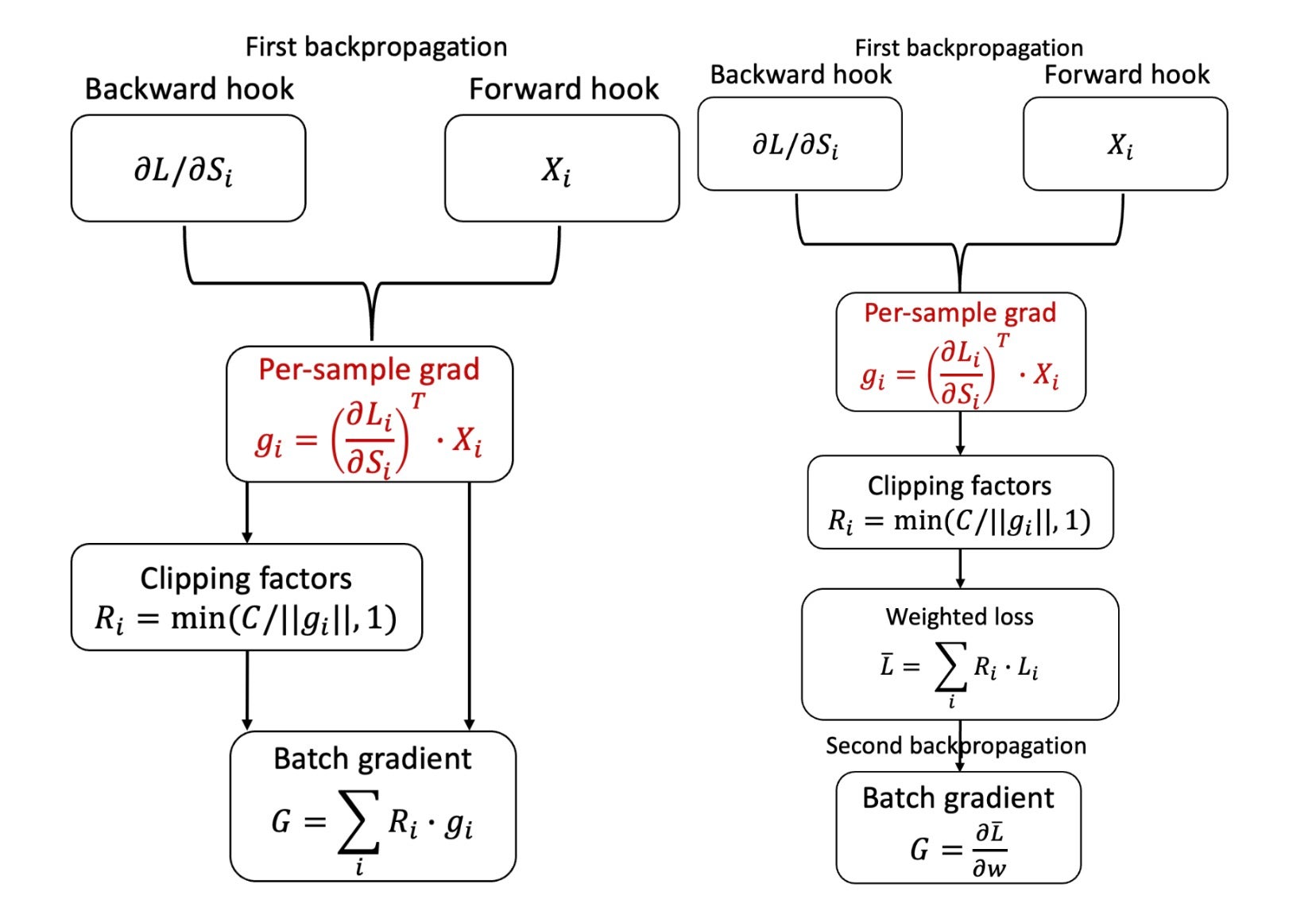
The key idea behind these techniques is based on the following observation: suppose per-sample gradient norms are known, then gradient clipping can be achieved by backpropagation on a re-weighted loss function $ \bar{L} $. This loss function is defined as $ \bar{L} = \sum_{i} R_{i} L_{i} $, where $ R_i = \min\left(\frac{C}{C_i}, 1\right) $ are the clipping coefficients computed from the per-sample gradient norms $ {C_i} $ and $ {L_i} $ are per-sample losses.
The above idea may seem circular at first glance, as it appears to require instantiating per-sample gradients in order to calculate per-sample gradient norms. However, for certain widely-used components of neural network architectures, such as fully connected/linear layers, it is indeed possible to obtain per-sample gradient norms in a single backpropagation pass without the need for per-sample gradients. This suggests a workflow that involves two backpropagation passes: the first to compute per-sample gradient norms, and the second to compute the aggregated (not per-sample) clipped gradient. The second backpropagation is simply the standard batched backpropagation.


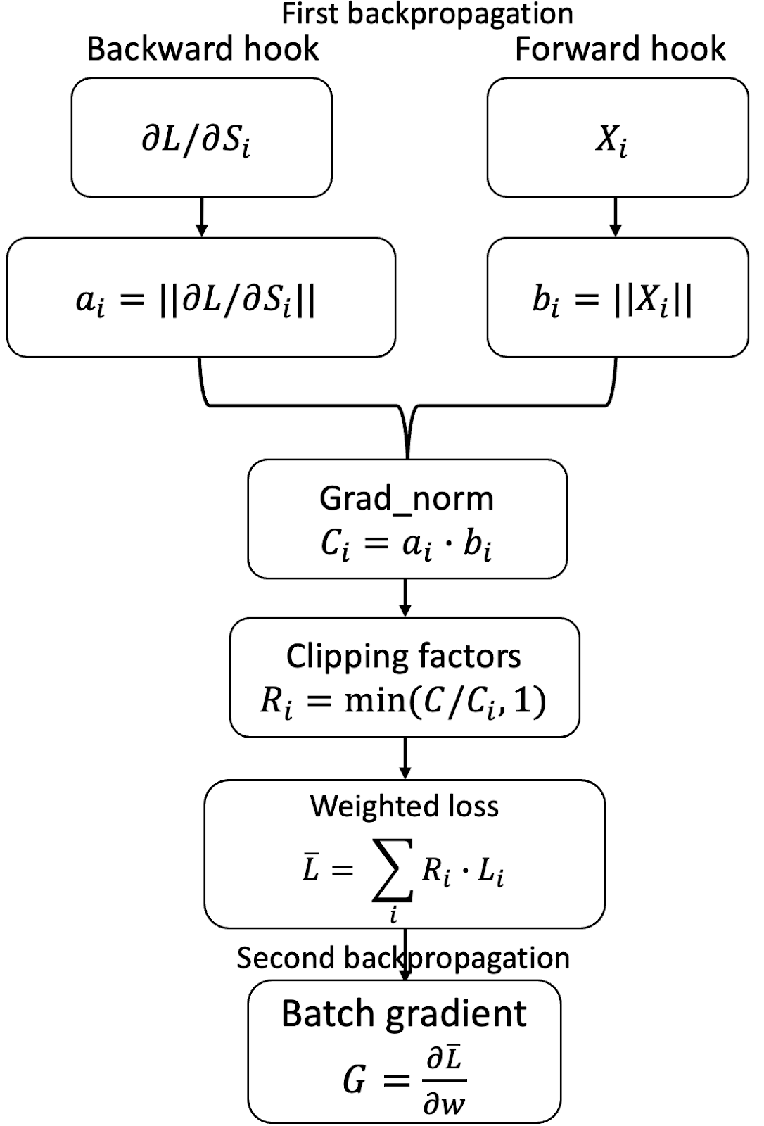
Figure 1: Comparison between vanilla Opacus (top left), Fast Gradient Clipping (top right), and Ghost clipping (bottom). We marked in red gradient instantiations that become memory bottlenecks. For vanilla Opacus, it has to instantiate the per-sample gradients. Fast Gradient Clipping instantiates per-sample gradients for each layer to compute its norm, which is immediately released once the backward pass moves on to the next layer. Ghost Clipping works directly from per-sample activation gradients and per-sample activations, and avoids the need for gradient instantiation.
Fast Gradient Clipping
In Fast Gradient Clipping, the per-sample gradient norm is calculated in three steps:
- For each layer, the per-sample gradient is instantiated and its norm is calculated.
- The per-sample gradient is then immediately discarded.
- The (squared) per-sample gradient norms of each layer are summed up to obtain the overall (squared) per-sample gradient norm.
Ghost Clipping
Extending the approach of Fast Gradient Clipping, Ghost Clipping uses the fact that for linear layers1, per-sample gradient norms can be calculated just from activation gradients and activations. In particular, let backprops and activations be per-sample activation gradients and activations, of dimensions batch_size ✕ output_width and batch_size ✕ input_width, respectively. The per-sample gradient is the outer product of the two, which takes O(batch_size ✕ input_width ✕ output_width) time and space.
The ghost clipping trick instead calculates the (squared) norm of backprops and activations, sample-wise, and takes their product, which gives the (squared) norm of the gradient. This takes O(batch-size ✕ (input_width + output_width)) time and takes O(batch-size) space to store. Since per-sample activation and per-sample activation gradients are already stored, additional memory is needed only for storing the norms.
Relationship between Fast Gradient Clipping and Ghost Clipping
- Fast Gradient Clipping and Ghost Clipping are complementary techniques. Fast Gradient Clipping can be applied to any type of layer, while Ghost Clipping is a strictly better technique for supported layers.
- Our implementation automatically switches to Fast Gradient Clipping when the layer is not supported by Ghost Clipping.
How to use Fast Gradient Clipping in Opacus
The training loop is identical to that of the standard PyTorch loop. As in Opacus before, we use the PrivacyEngine(), which “sanitizes” the model and optimizer. To enable Ghost Clipping, the argument grad_sample_mode="ghost" is used. Additionally, make_private() takes the loss criterion as an extra input and sanitizes it. This allows us to hide the two backward passes and the loss rescaling in between in loss.backward().
from opacus import PrivacyEngine
criterion = nn.CrossEntropyLoss() # example loss function

privacy_engine = PrivacyEngine()
model_gc, optimizer_gc, criterion_gc, train_loader, = privacy_engine.make_private(
        module=model,
        optimizer=optimizer,
        data_loader=train_loader,
        noise_multiplier=noise_multiplier
        max_grad_norm=max_grad_norm,
	 criterion=criterion,
        grad_sample_mode="ghost",
)

# The training loop below is identical to that of PyTorch

for input_data, target_data in train_loader:
    output_gc = model_gc(input_data) # Forward pass
    optimizer_gc.zero_grad()
    loss = criterion_gc(output_gc, target_data)
    loss.backward()
    optimizer_gc.step()  # Add noise and update the model
Internally, before the first pass, we enable the hooks, which allows us to capture layer-wise values corresponding to forward and backward calls. They are used to compute the per-sample gradient norms. We then compute the clipping coefficients, rescale the loss function and disable hooks, which lets us use the standard PyTorch backward pass.
Memory Complexity Analysis
Consider a multi-layer neural network with the following properties:
L: Number of layers
d: Maximum layer width
B: Batch size
K: Number of non-supported/non-linear layers
The memory overhead of DP-SGD with Ghost Clipping compared to plain (PyTorch) SGD is an additive O(BL), required to store the per-sample gradient norms for all layers. Further, if there is a non-supported layer (if K≥1), then there is an additional O(Bd2) memory to instantiate the gradient of that layer.
Memory Benchmarking
We provide results on the memory usage for a variety of settings.
Fine-Tuning BERT
We consider the problem of privately fine-tuning the last three layers of BERT for a text classification task. The base model has over 100M parameters, of which we fine-tune the last three layers, BertEncoder, BertPooler, and Classifier, comprising roughly 7.6M parameters. The experiments are run on a P100 GPU with 16 GB of memory.
The following table reports the maximum memory and time taken per iteration for the various methods:
| Batch size | |||||||||
| B = 32 | B = 128 | B = 512 | B = 1024 | B = 2048 | |||||
| Mem | Time | Mem | Time | Mem | Time | Mem | Time | ||
| PyTorch SGD | 236 MB | 0.15 s | 1.04 GB | 0.55 s | 5.27 GB | 2.1 s | 12.7 GB | 4.2 s | OOM |
| DP-SGD | 1,142 MB | 0.21 s | 4.55 GB | 0.68 s | OOM | OOM | OOM | ||
| FGC DP-SGD | 908 MB | 0.21 s | 3.6 GB | 0.75 s | OOM | OOM | OOM | ||
| GC DP-SGD | 362 MB | 0.21 s | 1.32 GB | 0.67 s | 5.27 GB | 2.5 s | 12.7 GB | 5 s | OOM |
In terms of peak memory footprint, DP-SGD > FGC DP-SGD ≫ GC DP-SGD ≈ PyTorch SGD. Further, the runtimes are similar because most of the parameters are frozen and the forward pass takes up most of the time.
Synthetic Setup: Memory Profiling
We consider the following setup to profile the memory used by PyTorch SGD, Vanilla DP-SGD and Ghost Clipping, GC DP-SGD.
- 2-layer fully connected neural network
- Input: 5120
- Hidden: 2560
- Output: 1280
- Total number of model parameters = 15.6M
- Model size = 62.5 MB
- Batch size, different values, as seen in the table below.
The table below summarizes the max memory increase (in MB) broken down by stages of the training loop for each of the methods.
| Batch Size | Method | Model to GPU | Forward | First Backward | Second Backward | Optimizer Step |
| 32 | PyTorch SGD | 62.5 | 0.5 | 62.5 | N/A | 0 |
| Vanilla DP-SGD | 62.5 | 0.47 | 3,663 | N/A | 162.5 | |
| GC DP-SGD | 62.5 | 0.47 | 63.13 | 50 | 125 | |
| 217 | PyTorch SGD | 62.5 | 1920 | 1932.5 | N/A | 0 |
| Vanilla DP-SGD | OOM | |||||
| GC DP-SGD | 62.5 | 1920 | 2625 | 1932.5 | 125 | |
Industry use case
We tested Ghost Clipping DP-SGD on an internal Meta use case, consisting of a model of size roughly 100B with 40M trainable parameters. Our initial results show that Ghost Clipping SGD reduces 95% memory of vanilla DP-SGD, and achieves comparable memory usage to PyTorch SGD.
Conclusion
In this post, we describe implementations of Fast Gradient Clipping and Ghost Clipping in Opacus that enable memory-efficient training of machine learning models with differential privacy. Currently, the Ghost Clipping implementation only applies to linear layers, but, as outlined in part 3 of the series, it can be extended to “generalized” linear layers such as convolutions and multi-head attention. The current techniques require two explicit backpropagation steps, which increases runtime. We will explore developments on top of Ghost Clipping such as the Book-Keeping algorithm for mitigation.
To learn more about Opacus, visit opacus.ai and github.com/pytorch/opacus.
Acknowledgements
We thank Iden Kalemaj, Darren Liu, Karthik Prasad, Hao Shi, Igor Shilov, Davide Testuggine, Eli Uriegas, Haicheng Wang, and Richard Zou for valuable feedback and suggestions.