Over the past year, we’ve added support for semi-structured (2:4) sparsity into PyTorch. With just a few lines of code, we were able to show a 10% end-to-end inference speedup on segment-anything by replacing dense matrix multiplications with sparse matrix multiplications.
However, matrix multiplications are not unique to neural network inference – they happen during training as well. By expanding on the core primitives we used earlier to accelerate inference, we were also able to accelerate model training. We wrote a replacement nn.Linear layer, SemiSparseLinear, that is able to achieve a 1.3x speedup across the forwards + backwards pass of the linear layers in the MLP block of ViT-L on a NVIDIA A100.
End-to-end, we see a wall time reduction of 6% for a DINOv2 ViT-L training, with virtually no accuracy degradation out of the box (82.8 vs 82.7 on ImageNet top-1 accuracy).
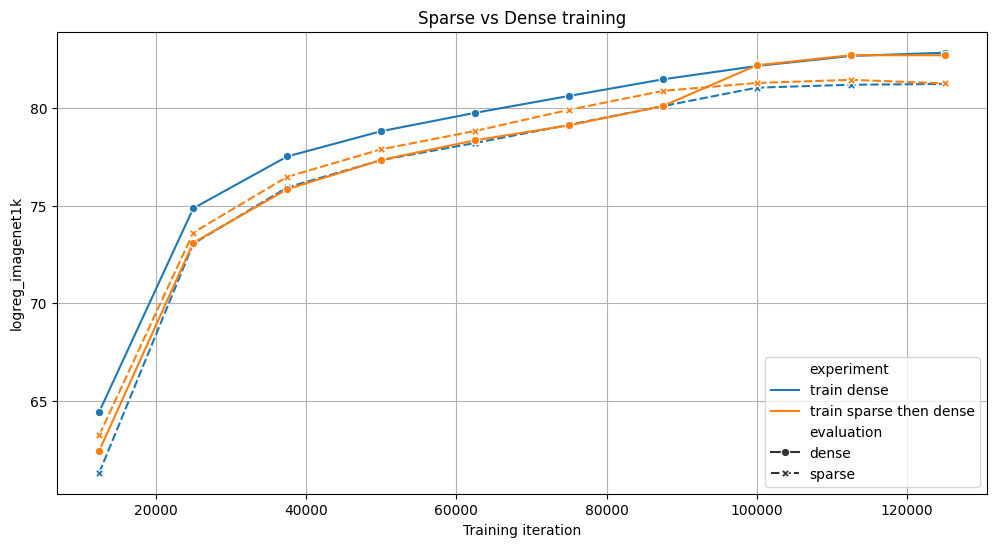
We compare 2 strategies for training a ViT model for 125k iterations on 4x NVIDIA A100s: either fully dense (blue), or sparse for 70% of the training, then dense (orange). Both achieve similar results on the benchmarks, but the sparse variant trains 6% faster. For both experiments, we evaluate the intermediate checkpoints with and without sparsity.
As far as we are aware, this is the first OSS implementation of accelerated sparse training and we’re excited to provide a user API in torchao. You can try accelerating your own training runs with just a few lines of code:
# Requires torchao and pytorch nightlies and CUDA compute capability 8.0+
import torch
from torchao.sparsity.training import (
    SemiSparseLinear,
    swap_linear_with_semi_sparse_linear,
)

model = torch.nn.Sequential(torch.nn.Linear(1024, 4096)).cuda().half()

# Specify the fully-qualified-name of the nn.Linear modules you want to swap
sparse_config = {
    "seq.0": SemiSparseLinear
}

# Swap nn.Linear with SemiSparseLinear, you can run your normal training loop after this step
swap_linear_with_semi_sparse_linear(model, sparse_config)
How does this work?
The general idea behind sparsity is simple: skip calculations involving zero-valued tensor elements to speed up matrix multiplication. However, simply setting weights to zero isn’t enough, as the dense tensor still contains these pruned elements and dense matrix multiplication kernels will continue to process them, incurring the same latency and memory overhead. To achieve actual performance gains, we need to replace dense kernels with sparse kernels that intelligently bypass calculations involving pruned elements.
These kernels work on sparse matrices, which remove the pruned elements and store the specified elements in a compressed format. There are many different sparse formats, but we’re particularly interested in semi-structured sparsity, also known as 2:4 structured sparsity or fine-grained structured sparsity or more generally N:M structured sparsity.
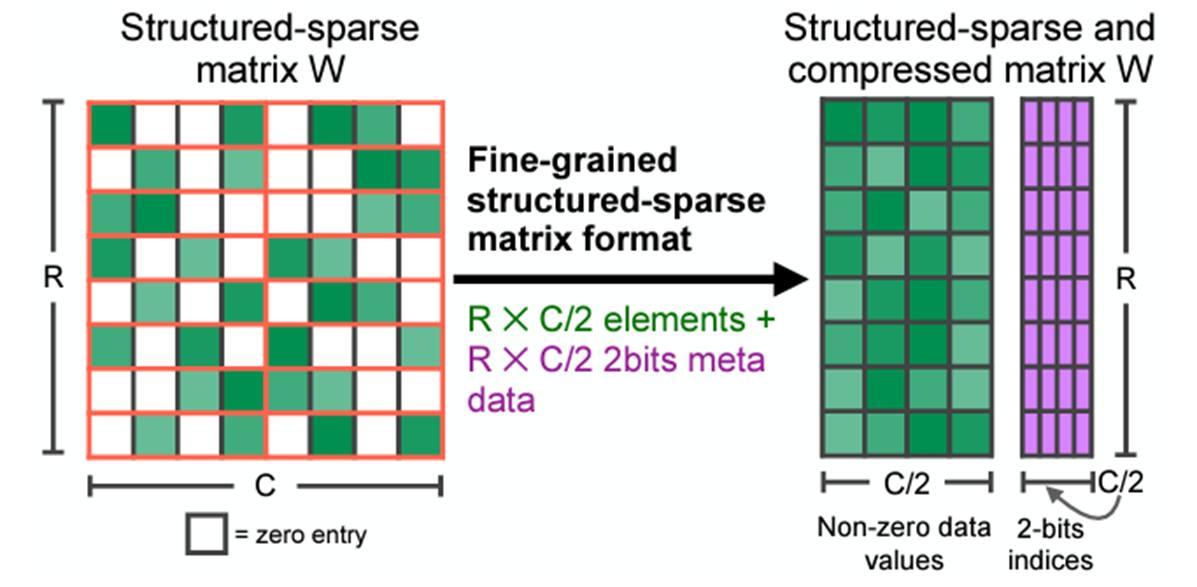
2:4 sparse compressed representation. Original Source
A 2:4-sparse matrix is a matrix where at most 2 elements are non-zero for every 4 elements, as illustrated in the image above. Semi-structured sparsity is attractive because it exists in a goldilocks spot of performance and accuracy:
- NVIDIA GPUs since Ampere offer hardware acceleration and library support (cuSPARSELt) for this format, with matrix multiplication being up to 1.6x faster
- Pruning models to fit this sparsity pattern does not degrade accuracy as much as other patterns. NVIDIA’s whitepaper shows pruning then retraining is able to recover accuracy for most vision models.
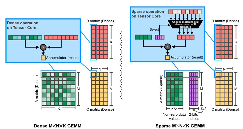
Illustration of 2:4 (sparse) matrix multiplication on NVIDIA GPUs. Original source
Accelerating inference with semi-structured sparsity is straightforward. Since our weights are fixed during inference, we can prune and compress the weight ahead of time (offline) and store the compressed sparse representation instead of our dense tensor.
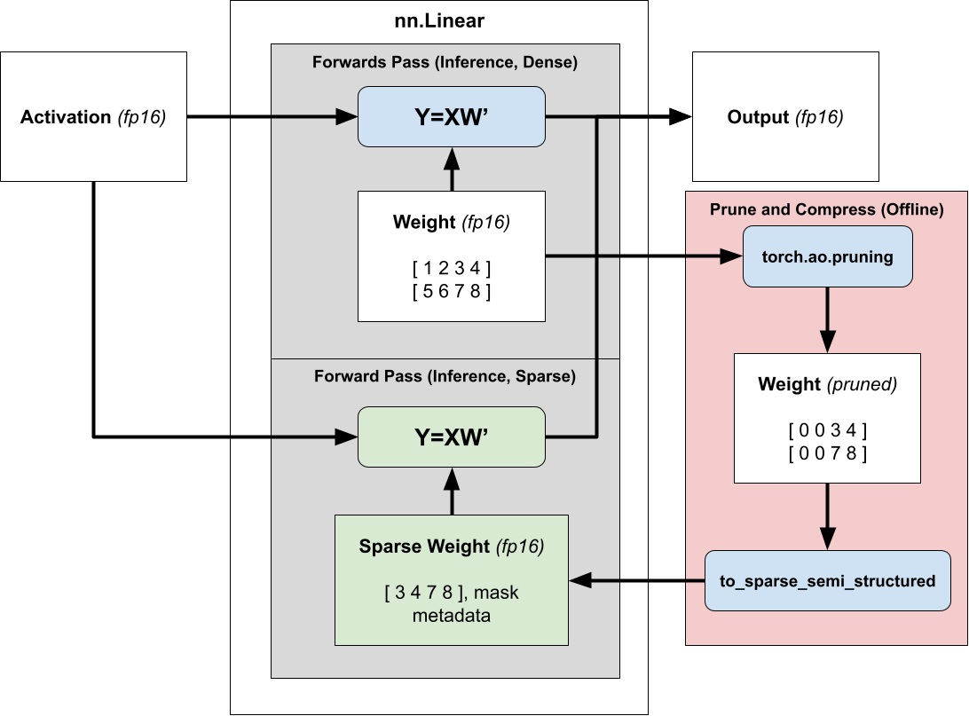
Then, instead of dispatching to dense matrix multiplication we dispatch to sparse matrix multiplication, passing in the compressed sparse weight instead of the normal dense one. For more information about accelerating models for inference using 2:4 sparsity, please refer to our tutorial.
Extending sparse inference acceleration to training
In order to use sparsity to reduce the training time of our models, we need to consider when the mask is calculated, as once we store the compressed representation the mask is fixed.
Training with a fixed mask applied to an existing trained dense model (also known as pruning) does not degrade accuracy, but this requires two training runs – one to obtain the dense model and another to make it sparse, offering no speedups.
Instead we’d like to train a sparse model from scratch (dynamic sparse training), but training from scratch with a fixed mask will lead to a significant drop in evaluations, as the sparsity mask would be selected at initialization, when the model weights are essentially random.
To maintain the accuracy of the model when training from scratch, we prune and compress the weights at runtime, so that we can calculate the optimal mask at each step of the training process.
Conceptually you can think of our approach as an approximate matrix multiplication technique, where we `prune_and_compress` and dispatch to `sparse_GEMM` in less time than a `dense_GEMM` call would take. This is difficult because the native pruning and compression functions are too slow to show speedups.
Given the shapes of our ViT-L training matrix multiplications (13008x4096x1024), we measured the runtime of a dense and sparse GEMM respectively at 538us and 387us. In other words, the pruning and compression step of the weight matrix must run in less than 538-387=151us to have any efficiency gain. Unfortunately, the compression kernel provided in cuSPARSELt already takes 380us (without even considering the pruning step!).
Given the max NVIDIA A100 memory IO (2TB/s), and considering that a prune and compress kernel would be memory bound, we could theoretically prune and compress our weight (4096x1024x2 bytes=8MB) in 4us (8MB / 2TB/s)! And in fact, we were able to write a kernel that prunes and compresses a matrix into 2:4-sparse format, and runs in 36 us (10x faster than the compression kernel in cuSPARSELt), making the entire GEMM (including the sparsification) faster. Our kernel is available for use in PyTorch.
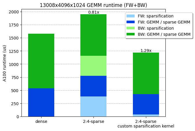
Our custom sparsification kernel, which includes pruning + compression, is ~30% faster across a linear layer forward+backward. Benchmarks run on a NVIDIA A100-80GB GPU.
Writing a performant runtime sparsification kernel
There were multiple challenges we faced in order to implement a performant runtime sparsification kernel, which we will explore below.
1) Handling the backwards pass
For the backwards pass, we need to calculate dL/dX and dL/dW for the gradient update and the subsequent layer, which means we need to calculate xWT and xTW respectively.
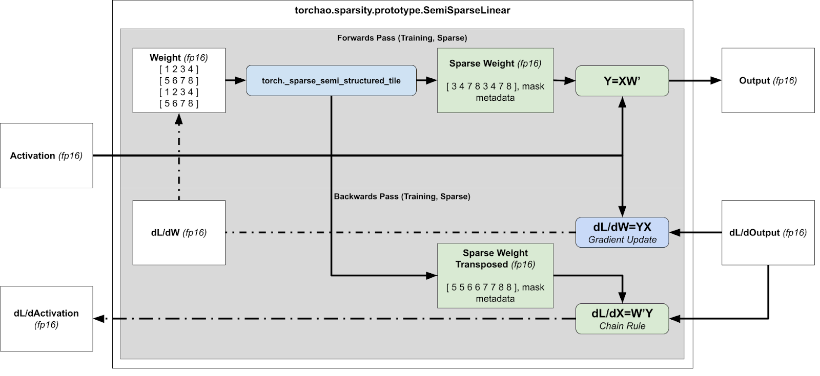
Overview of runtime sparsification for training acceleration (FW + BW pass)
However this is problematic, because the compressed representation cannot be transposed, since there’s no guarantee that the tensor is 2:4 sparse in both directions.

Both matrices are valid 2:4 matrices. However, the right one is no longer a valid 2:4 matrix once transposed because one column contains more than 2 elements
Therefore, we prune a 4×4 tile, instead of a 1×4 strip. We greedily preserve the largest values, ensuring that we take at most 2 values for each row / column. While this approach is not guaranteed to be optimal, as we sometimes only preserve 7 values instead of 8, it efficiently calculates a tensor that is 2:4 sparse both row-wise and column-wise.
We then compress both the packed tensor and the packed transpose tensor, storing the transpose tensor for the backwards pass. By calculating both the packed and packed transpose tensor at the same time, we avoid a secondary kernel call in the backwards pass.
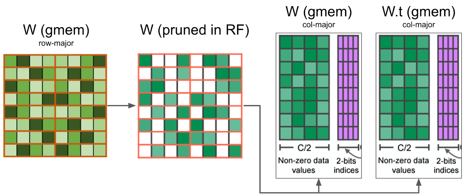
Our kernel prunes the weight matrix in registers, and writes the compressed values in global memory. It also prunes at the same time W.t, which is needed for the backward pass, minimizing the memory IO
There’s some additional transpose trickery needed to handle the backwards pass – the underlying hardware only supports operations where the first matrix is sparse. For weight sparsification during inference, when we need to calculate xWT we rely on transpose properties to swap the order of the operands.
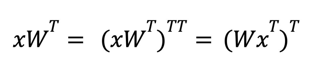
During inference, we use torch.compile to fuse the outer transpose into subsequent pointwise ops in order to avoid paying a performance penalty.
However in the case of the backwards pass of training, we have no subsequent pointwise op to fuse with. Instead, we fuse the transposition into our matrix multiplication by taking advantage of cuSPARSELt’s ability to specify the row / column layout of the result matrix.
2) Kernel tiling for efficient memory-IO
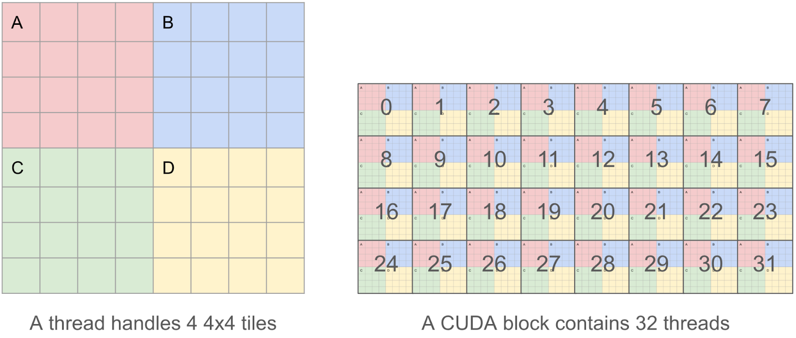
In order for our kernel to be as efficient as possible, we want to coalesce our reads / writes, as we found that memory IO to be the main bottleneck. This means that within a CUDA thread, we want to read/write chunks of 128 bytes at a time, so that multiple parallel reads/writes can be coalesced into a single request by the GPU memory controller.
Therefore, instead of a thread handling a single 4×4 tile, which is only 4x4x2 = 32 bytes, we decided that each thread will handle 4 4×4 tiles (aka an 8×8 tile), which allows us to operate 8x8x2 =128 byte chunks.
3) Sorting elements in a 4×4 tile without warp-divergence
For each individual 4×4 tile within our thread we calculate a bitmask that specifies which elements to prune and which elements to keep. To do this we sort all 16 elements and greedily preserve elements, so long as they do not break our 2:4 row / col constraint. This preserves only the weights with the largest values.
Crucially we observe that we are only ever sorting a fixed number of elements, so by using a branchless sorting network, we can avoid warp divergence.
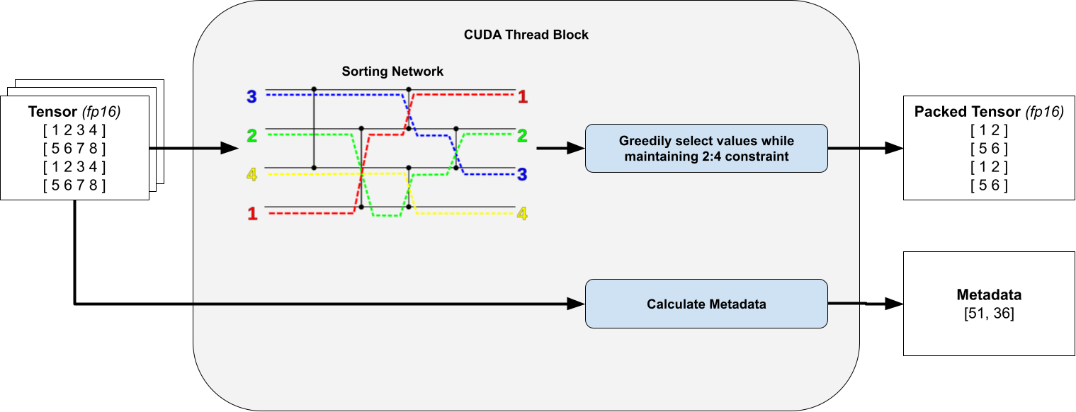
For clarity, the transposed packed tensor and metadata are omitted. Sorting network diagram taken from Wikipedia.
Warp divergence occurs when we have conditional execution inside across a thread block. In CUDA, work items in the same work group (thread block) are dispatched at the hardware level in batches (warps). If we have conditional execution, such that some work-items in the same batch run different instructions, then they are masked when the warp is dispatched, or dispatched sequentially.
For example, if we have some code like if (condition) do(A) else do(B), where condition is satisfied by all the odd-numbered work items, then the total runtime of this conditional statement is do(A) + do(B), since we would dispatch do(A) for all odd-numbered work-items, masking out even-numbered work-items, and do(B) for all even numbered work-items, masking out odd-numbered work-items. This answer provides more information about warp divergence.
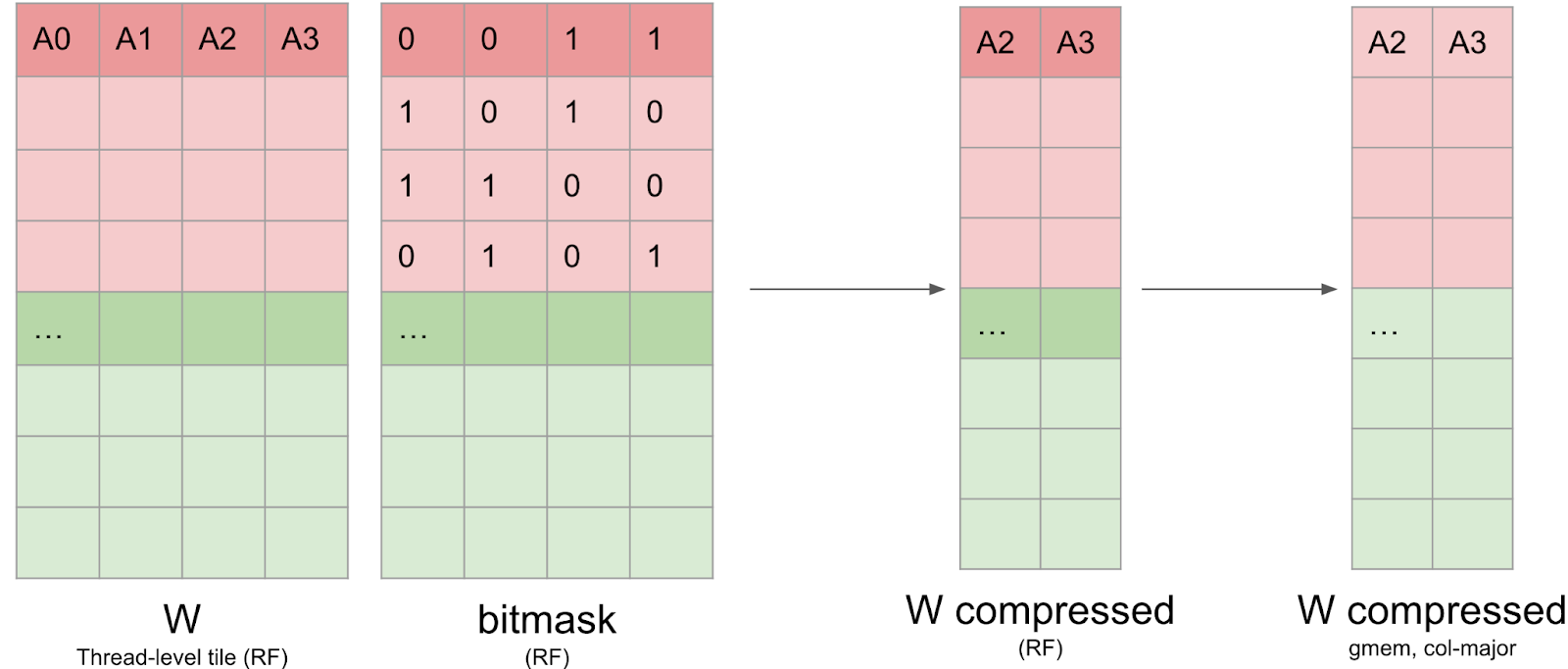
4) Writing the compressed matrices and metadata
Once the bitmask has been computed, the weight data has to be written back in a compressed format in global memory. This is not trivial, because the data needs to stay in registers, and it’s not possible to index registers (eg C[i++] = a prevents us from storing C in registers). Furthermore, we found that nvcc was using many more registers than we expected, which caused register spilling and impacted global performance. We write this compressed matrix to global memory in Column-Major format to make the writes more efficient.
We also need to write the cuSPARSELt metadata as well. This metadata layout is quite similar to the one from the open-source CUTLASS library and is optimized for being loaded efficiently through shared-memory in the GEMM kernel with the PTX ldmatrix instruction.
However, this layout is not optimized to be written efficiently: the first 128 bits of the metadata tensor contains metadata about the first 32 columns of the rows 0, 8, 16 and 24. Recall that each thread handles an 8×8 tile, which means that this information is scattered across 16 threads.
We rely on a series of warp-shuffle operations, once for the original and transposed representation respectively to write the metadata. Fortunately, this data represents less than 10% of the total IO, so we can afford to not fully coalesce the writes.
DINOv2 Sparse Training: Experimental Setup and Results
For our experiments, the ViT-L model is trained on ImageNet for 125k steps using the DINOv2 method. All our experiments were run on 4x AMD EPYC 7742 64-core CPUs and 4x NVIDIA A100-80GB GPUs. During sparse training, the model is trained with 2:4 sparsity enabled for the first part of the training, where only half of the weights are enabled. This sparsity mask on the weights is dynamically recomputed at every step, as weights are continuously updated during the optimization. For the remaining steps, the model is trained densely, producing a final model without 2:4 sparsity (except the 100% sparse training setup), which is then evaluated.
| Training setup | ImageNet 1k log-regression |
| 0% sparse (125k dense steps, baseline) | 82.8 |
| 40% sparse (50k sparse -> 75k dense steps) | 82.9 |
| 60% sparse (75k sparse -> 50k dense steps) | 82.8 |
| 70% sparse (87.5k sparse -> 37.5k dense steps) | 82.7 |
| 80% sparse (100k sparse -> 25k dense steps) | 82.7 |
| 90% sparse (112.5k sparse -> 12.5k dense steps) | 82.0 |
| 100% sparse (125k sparse steps) | 82.3 (2:4-sparse model) |
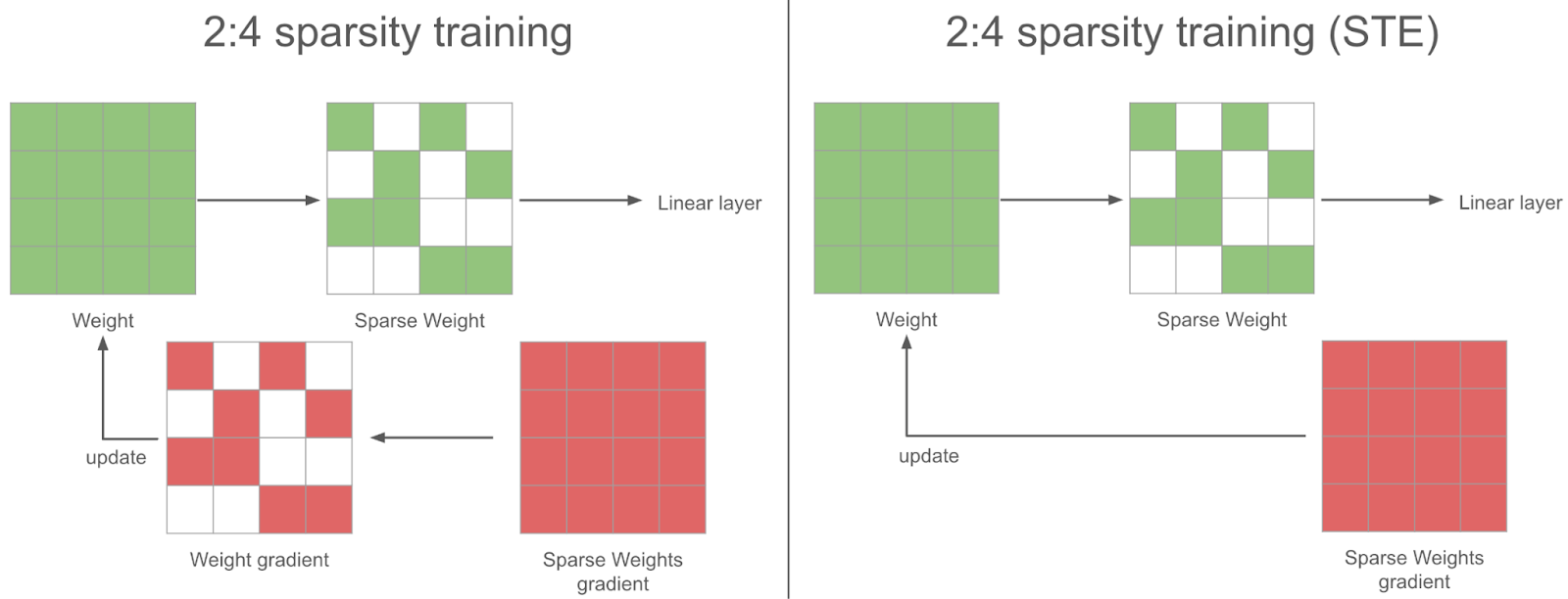
During the sparse training steps, in the backward pass we obtain a dense gradient for the sparse weights. For the gradient descent to be sound, we should also sparsify this gradient before using it in the optimizer to update the weights. Instead of doing that, we use the full dense gradient to update the weights – we found this to work better in practice: this is the STE (Straight Through Estimator) strategy. In other words, we update all the parameters at every step, even the ones we don’t use.
Conclusion and Future Work
In this blog post, we’ve shown how to accelerate neural network training with semi-structured sparsity and explained some of the challenges we faced. We were able to achieve a 6% end to end speedup on DINOv2 training with a small 0.1 pp accuracy drop.
There are several areas of expansion for this work:
- Expansion to new sparsity patterns: Researchers have created new sparsity patterns like V:N:M sparsity that use the underlying semi-structured sparse kernels to allow for more flexibility. This is especially interesting for applying sparsity to LLMs, as 2:4 sparsity degrades accuracy too much, but we have seen some positive results for more general N:M pattern.
- Performance optimizations for sparse fine-tuning: This post covers sparse training from scratch, but oftentimes we want to fine-tune a foundational model. In this case, a static mask may be sufficient to preserve accuracy which would enable us to make additional performance optimizations.
- More experiments on pruning strategy: We calculate the mask at each step of the network, but calculating the mask every n steps may yield better training accuracy. Overall, figuring out the best strategy to use semi-structured sparsity during training is an open area of research.
- Compatibility with fp8: The hardware also supports fp8 semi-structured sparsity, and this approach should work similarly with fp8 in principle. In practice, we would need to write similar sparsification kernels, and could possibly fuse them with the scaling of the tensors.
- Activation Sparsity: Efficient sparsification kernels also enable to sparsify the activations during training. Because the sparsification overhead grows linearly with the sparsified matrix size, setups with large activation tensors compared to the weight tensors could benefit more from activation sparsity than weight sparsity. Furthermore, activations are naturally sparse because of the usage of ReLU or GELU activation functions, reducing accuracy degradation.
If you are interested in these problems, please feel free to open an issue / PR in torchao, a community we’re building for architecture optimization techniques like quantization and sparsity. Additionally, if you have general interest in sparsity please reach out in CUDA-MODE (#sparsity)