Accelerating Mamba2 with Kernel Fusion

Summary

In this post, we discuss how we optimized the Mamba-2 State-Space Dual (SSD) module with a fused Triton kernel that yields speedups of 1.50x-2.51x on NVIDIA A100 and H100 GPUs. To achieve this, we fused all five SSD kernels into a single Triton kernel with careful synchronization. To our knowledge, this is the first end-to-end Triton fusion of all five SSD kernels. This reduces launch overhead and avoids redundant memory operations, making the kernel faster across all input sizes. The rest of this blog will cover how we fused the SSD kernels, what bottlenecks remain, benchmark results, and our plans to release the kernel in the open source so the community can benefit.

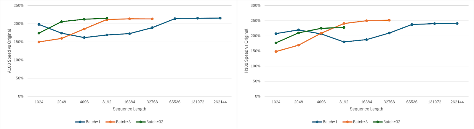
Figure 1. Fused SSD Triton Kernel A100 and H100 Speedups

Background

Mamba-2 is a sequence model based on the state-space duality (SSD) framework, which connects structured state-space models (SSMs) with attention-based transformers as an optimized successor to the original Mamba model. One key advantage of Mamba-style models is scalability to long sequences. Mamba’s state-space mechanism scales linearly with context length. In practice, doubling the input sequence length roughly doubles Mamba’s compute and memory needs, whereas self-attention would quadruple them. This makes Mamba-2 especially attractive for extremely long contexts, such as 128K tokens and beyond.

IBM’s Granite 4.0 model family recently adopted a hybrid architecture that combines Mamba-2 blocks with transformer blocks. In Granite 4.0, nine Mamba-2 layers are used for every one attention layer to handle long-range context efficiently. With Mamba-2 becoming integral to such models, optimizing Mamba-2’s performance is critical for faster inference. The core of Mamba-2’s computation is the SSD module, which replaces the attention mechanism in each layer. The original Mamba2 SSD implementation is mostly bottlenecked by memory bandwidth and latency and includes writing and reading intermediate data, so there are opportunities for improvement. In this blog, we focus on accelerating this SSD prefill operation with an optimized fused kernel.

Mamba2 Operations

The operations that make up a typical Mamba2 block are listed in Table 1. We focused on fusing the five SSD kernels because they behave as one conceptual SSD operation, though further fusion (e.g., convolution and layernorm) may be possible as discussed later.

 

Layernorm	Helps with numerical stability
In Projection	Projects input to SSD channels/size
Depthwise Convolution	Mixes the last few tokens
SSD Chunk Cumsum	Computes the dt per token and cumulative decay within a chunk
SSD Chunk State	Computes the state at the end of this chunk in isolation
SSD State Passing	Computes the global states at the end of each chunk
SSD BMM	Computes how the each chunk of input x affects the corresponding chunk of output y
SSD Chunk Scan	Computes each chunk of y from the corresponding chunk of x and previous chunk’s global state
Layernorm	Helps with numerical stability
Out Projection	Projects output to the model’s hidden dim

Table 1. Mamba2 operations

Why Do We Need Kernel Fusion?

During prefill, which is the forward pass over the prompt or input sequence before token generation, Mamba-2’s SSD module executes as a pipeline of five GPU kernels. In the original implementation, these five kernels run sequentially on the GPU.
However, launching multiple small kernels in sequence incurs significant overhead and prevents the GPU from reusing data between stages efficiently. By applying kernel fusion we can get several key benefits:

• Eliminating Kernel Launch Overheads: One launch instead of five reduces CPU-GPU synchronization and scheduling delays.
• Improving Cache Locality: Data produced in one stage is immediately consumed by the next within the same threadblock, increasing cache hits and reducing global memory traffic.
• Overlapping Computation: Different parts of the fused kernel can execute in parallel (where independent), better utilizing GPU resources.

Our solution fuses all five kernels into a single Triton kernel, so that the entire SSD prefill computation for a layer happens within one GPU launch.

Efficient Kernel Fusion Technique

Unlike a simple matmul + activation fusion, SSD fusion is complex because the computation spans multiple steps with complicated dependencies. The original implementation relied on implicit synchronization across kernels, which disappears when we fuse everything. In this section, we discuss why that matters and our approach to making fusion work in practice.

The five steps of the Mamba2 SSD were originally implemented as five separate kernels: Chunk Cumsum, BMM, Chunk State, State Passing, and Chunk Scan, which operate on fixed-size chunks of tokens. The figure below illustrates the dependencies between these kernels.

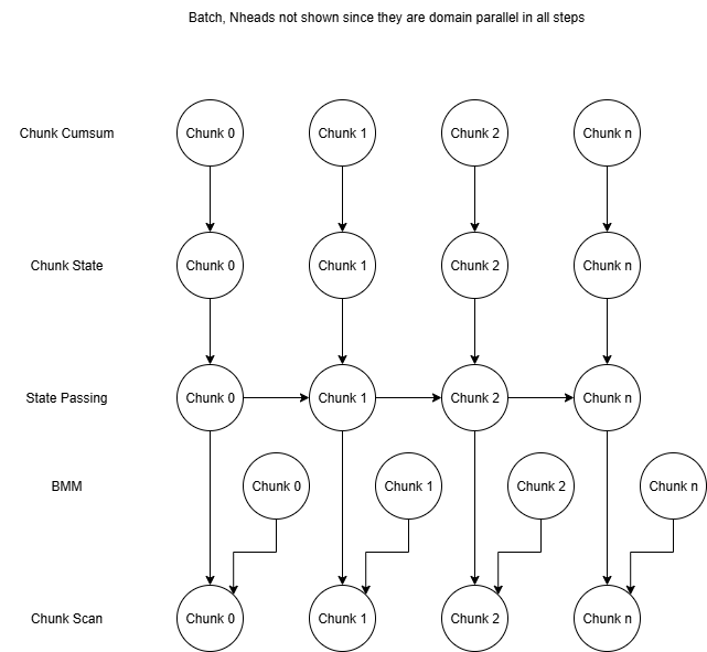
Figure 2. Mamba2 SSD Prefill Kernel Graph

The State Passing step has dependencies between chunks, and the original State Passing kernel handled this by looping over chunks within threadblocks and splitting the state’s channels across threadblocks for parallelism. With this State Passing loop and the implicit global synchronization between kernel launches, all dependencies were handled in the original kernels.

The real technical challenge comes when we try to fuse all five kernels into a single launch. Once fused, we lose the implicit global synchronization that the original kernels relied on, so we must explicitly manage both within-chunk and across-chunk dependencies. Most of the dependencies are between different steps but the same chunk, so for the three largest kernels, Chunk State, State Passing, and Chunk Scan, these intra-chunk dependencies could be handled by running all steps of a particular chunk on the same threadblock. This would also give us the ability to keep intermediate data between steps in registers or L1 cache (private to each SM) since the data will be used on the same threadblock.

However, this approach is neither possible nor correct. The original State Passing kernel has the aforementioned loop, which makes its threadblock grid not match the original Chunk State and Chunk Scan kernels. Furthermore, having separate threadblocks for each chunk would remove the natural synchronization and correctness provided by looping over chunks within a single threadblock.

To make fusion possible, we split the iterations of the State Passing loop across chunks into separate threadblocks so the threadblock grids match. We get correctness by ordering these threadblocks with atomics, a form of serialization that looks quite inefficient on the surface but can be mitigated by overlapping with the other two parts.

For example, if we ran 8 chunks in parallel, we would expect a ~8x local slowdown from the State Passing serialization. However, the fused State Passing is a small fraction of the three large steps, especially since it no longer has to read the state from global memory (it’s already in the threadblock from the fused Chunk State).

By Amdahl’s law, we would expect the runtime to change to (State Passing fraction) * 8 + (1 – State Passing fraction) * 1. For example, if the State Passing step was only 1/7th of the combined time excluding synchronization, we would get (1/7) * 8 + (6/7) * 1 = 2, implying a 2x overall slowdown. However, this does not account for overlap. Since the synchronization of State Passing can overlap with the Chunk State and Chunk Scan computation, the slowdown would be roughly: 

State Passing compute time + max(other compute time, State Passing synchronization time)

= 1/7 + max(6/7, 1/7 * 7) = 1.14x

If State Passing was a smaller fraction of the total runtime or if less chunks are processed concurrently, we could theoretically avoid any serialization slowdown in all but the first chunks.

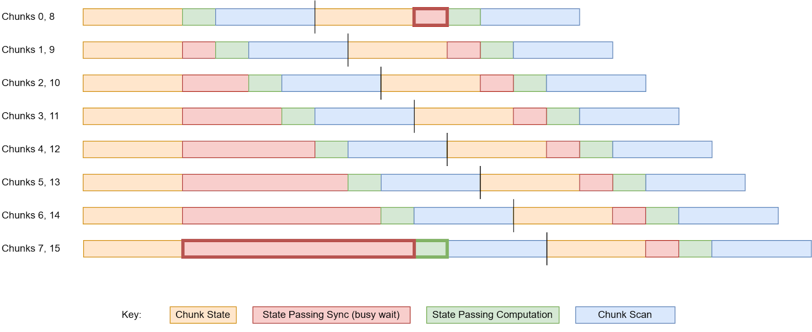
Figure 3. State Passing Overhead Overlap

Figure 3 shows the theoretical synchronization delays, which are high for the first chunks run in parallel, but settle down to a low overhead in all later chunks. We can see that although chunk 8 depends on chunk 7, it only has to busy-wait 1 unit of time instead of 8 since the chunk 0 Chunk Scan and chunk 8 Chunk State overlap with the State Passing of chunks 1-6. In practice, NVIDIA Nsight Compute benchmarks show that fewer than 3% of warp stalls (idle thread time) are caused by the State Passing synchronization, implying that the serialization latency is hidden.

The BMM and Chunk Cumsum steps are extremely fast compared to the other three. BMM splits work along ngroups instead of nheads, and Chunk Cumsum has its threadblocks handle multiple heads for efficiency. For simplicity, we launch separate threadblocks for these two steps (the first few threadblocks work on them) and have the threadblocks for the other three steps await their BMM and Chunk Cumsum dependencies with atomics.

When a threadblock begins executing the kernel, it is assigned to work on the Chunk Cumsum step unless all Chunk Cumsum work has already been assigned. Similarly, if there is no unassigned Chunk Cumsum work, the threadblock would be assigned to the BMM step if available. After both of these fast steps have been fully assigned to threadblocks, later threadblocks each start processing a chunk in Chunk State, process that same chunk in State Passing, and finally output that chunk after Chunk Scan.

While kernel fusion improves data reuse and speeds up the SSD, additional optimizations are necessary to achieve maximum performance. These include reordering threadblocks to hide serialization latency, adding cache hints to loads/stores to prioritize reused data, separating special cases outside of the fused kernel to reduce register pressure, changing some intermediate datatypes, tuning the chunk size, and restructuring operations for less latency. These optimization techniques are described in more detail in Appendix A.

Remaining Bottlenecks

In this section, we analyze the bottlenecks in the optimized fused SSD kernel using Nsight Compute to examine the final utilization, stall patterns, and resource tradeoffs.

At a high level, we can look at the compute and memory utilization of the fused kernel to get an idea of what limits this kernel.

Figure 4. A100 Nsight Compute Summary

Figure 5. H100 Nsight Compute Summary

We can see that overall fused SSD compute utilization is about 40-50% and memory utilization is about 65-75%. It is not possible to achieve 100% utilization due to the initial load/store latency and other overheads, but it’s usually possible to get at least 80% in a well-optimized kernel. For context, the H100 and A100 matmuls used in Mamba2 get 85-96% compute utilization. Since neither compute nor memory has good utilization in the SSD kernel, the bottlenecks are more complicated than just memory bandwidth or compute throughput.

We can look at the warp state statistics to see what warps are stalled on. “Selected” means that the warp executed a new instruction, but “Stall Long Scoreboard” and “Stall Barrier” indicate that warps are idle waiting for L2/VRAM or synchronizing.

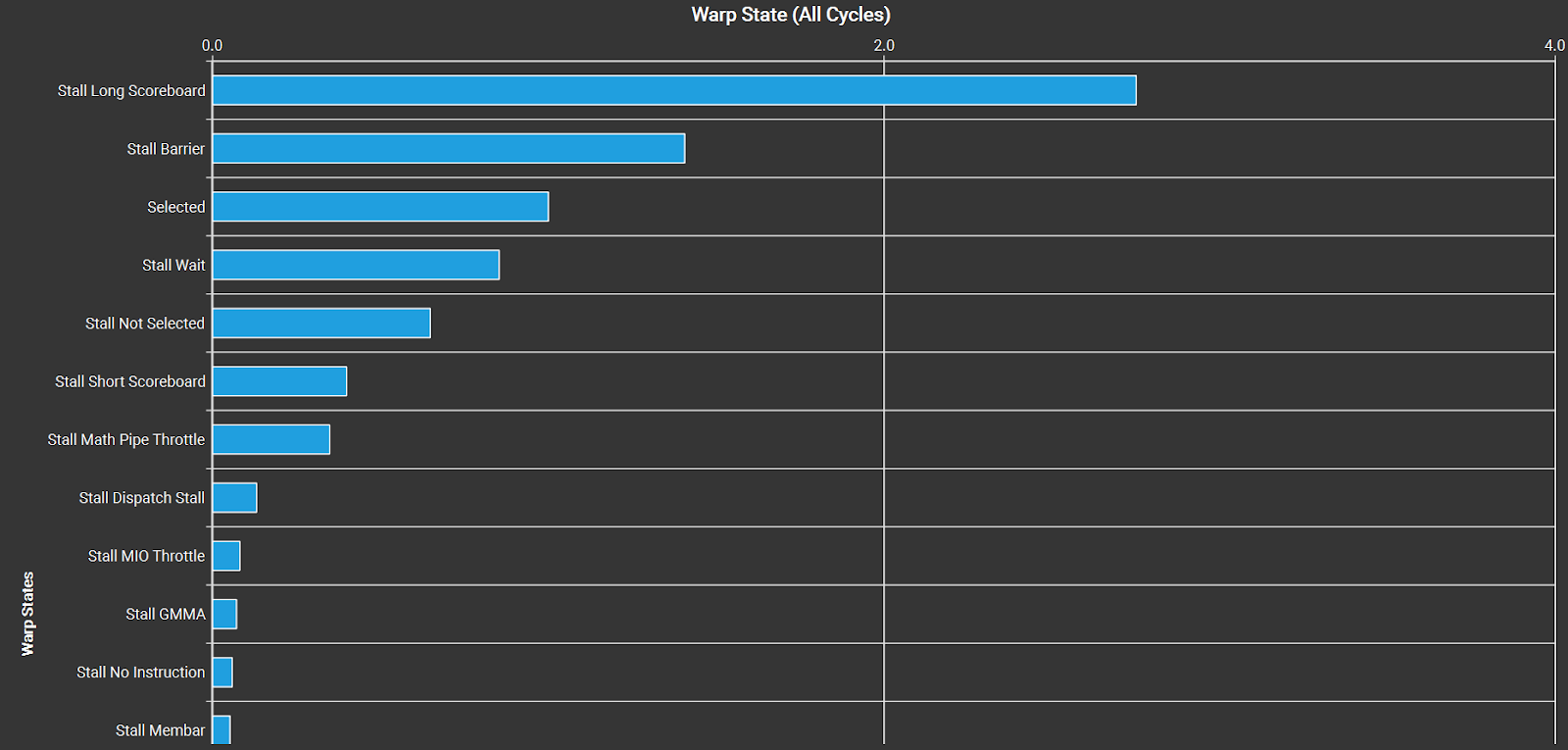
Figure 6. Warp State Statistics for the fused SSD kernel on an H100

There are a few ways to reduce the effect of these stalls and improve the compute or memory utilization:

1. Increase occupancy
2. Increase instruction-level parallelism
3. Optimize the code to use less synchronization and memory ops or cache data better

Occupancy

Modern NVIDIA GPUs have 12-16 warps (groups of 32 threads) per warp scheduler, and each of these warp schedulers can issue a new instruction every cycle. If we only have 1 warp in each scheduler, we waste cycles every time that the warp stalls. However, if we have 16 warps in each scheduler, each warp could be stalled about 15/16 of the time without leaving the hardware idle. Occupancy is the fraction of available warp slots that are actually filled with active warps. Increasing occupancy helps hide memory and instruction latency, increasing GPU utilization.

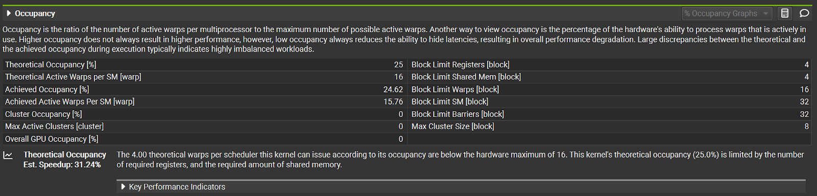
Figure 7. Occupancy for the fused SSD kernel on an H100

This fused kernel only gets 25% occupancy in the current config, limited by registers and shared memory. Although we can increase the number of warps and reduce the registers per thread to increase occupancy, this reduces performance in practice, likely due to increased synchronization costs and higher register pressure.

Instruction-Level Parallelism

Instruction-Level Parallelism means designing/optimizing the code to have less immediate dependencies between instructions, allowing the warp to run future instructions even when the previous instructions haven’t finished. This provides the same latency-hiding benefit as increased occupancy, but without requiring more warps.

Reducing Synchronization and Data Transfer

Since the warps are usually waiting on loading/storing memory or a barrier, we can improve performance by reducing the amount of barriers or reducing total data transfer through better caching or different block sizes.

Unfortunately, these three optimization techniques can directly clash and introduce tradeoffs. Each SM in the GPU has limited registers and shared memory, so if each threadblock uses too much, occupancy drops. We can increase instruction-level parallelism by loading data in stages, but that requires more registers and shared memory, resulting in lower occupancy. We can also change block sizes to reduce the total data transferred or increase the cache hit rates, but this also requires more resources and reduces occupancy.

This is why the fused kernel does not have very high memory or compute utilization.

Memory Utilization Details

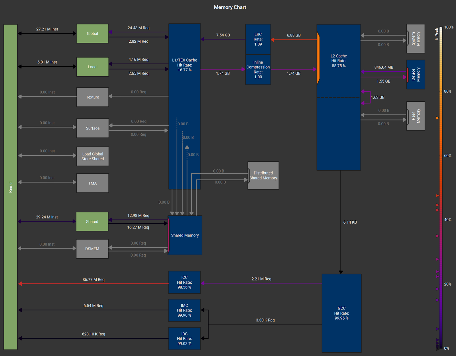
Figure 8. Memory Chart for the fused SSD kernel on an H100

We can see from this chart that the reported 65–75% memory utilization is mostly from reads through the L2 cache. These reads likely include (i) tensors that fit in L2, (ii) tensors reused across multiple threadblocks, (iii) state transfers between threadblocks, and (iv) VRAM reads that naturally pass through L2. Since L1 caches are private to each SM and not coherent across threadblocks, shifting this traffic to L1 is not feasible. Similarly, bypassing L2 for VRAM traffic would not help, as all global memory accesses pass through L2. 

This memory chart suggests that, apart from the suboptimal memory utilization, the kernel is effectively L2-bound rather than DRAM-bound. Further optimization would therefore require either (1) increasing memory utilization, (2) tuning the block sizes / config, or (3) making radical algorithmic changes.

Line-by-Line Stalls

Nsight Compute profiling shows warp stalls line-by-line, helping us check that the warp stalls are for legitimate reasons. As expected, most warp stalls in the fused kernel are from loading data, synchronization, and computation, with only minor overheads from atomics and inter-chunk synchronization. See Appendix B for more details.

Benchmarks

We benchmarked our Triton kernel on typical inference scenarios, batch size 1-32, sequence lengths from 1K up to 256K tokens, and fp16 states. These graphs highlight the speedup of our kernel over the baseline unfused kernels.

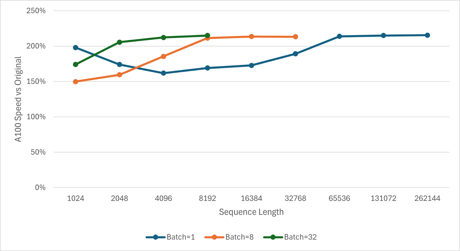
Figure 9. NVIDIA A100 Fused Kernel Speedup Graph

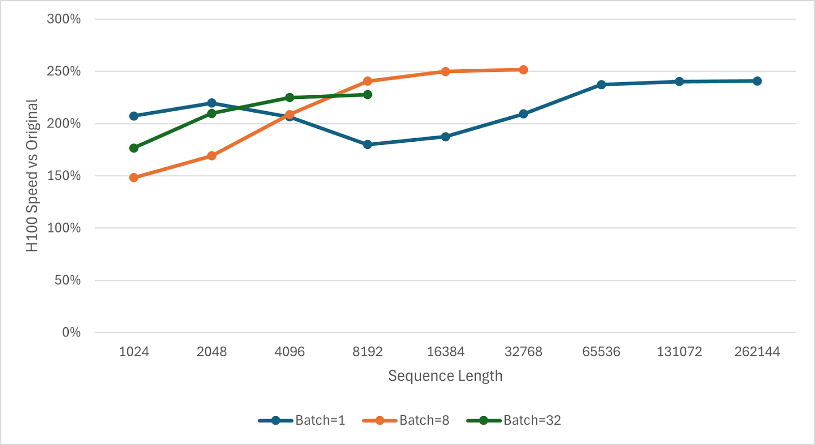
Figure 10. NVIDIA H100 Fused Kernel Speedup Graph

The fused SSD kernel is 1.50x-2.51x faster than the unfused implementation on the SSD portion. At low sequence lengths (especially with batch=1), overheads from kernel launches help the fused kernel, but these constant costs become amortized for longer sequences. At higher sequences, the fused kernel’s lower data movement is even more beneficial as cache thrashing increases. The SSD speedup translates to roughly a 8-13% end-to-end speedup for a model like Mamba-2 2.7B with batch=1 and seq=128K on NVIDIA A100 and H100 GPUs. At shorter sequence lengths, the end-to-end speedup can reach ~20% at 1K context, likely due to the reduced kernel launch overhead.

Accuracy and Correctness

The fused kernel is generally accurate and correct, but there are slight differences in output between the fused kernel and reference solution. These differences depend on the GPU it’s running on and the precisions of some computations. The fused kernel internally uses fp16 for some computations that the original kernels used fp32 for, because this gives a ~16% speedup. Furthermore, the original kernels support either fp32 or fp16 states, but our reported speedups are for fp16 states. The fused kernel still supports the same intermediate datatypes and fp32 states. In this section we explain the tradeoffs in accuracy and performance for these different dtype configs.

In Table 2, we report the accuracy of the output y tensor as percentage of elements that match the original kernels’ output. We test with no threshold (element must exactly match), a small threshold of 1e-3 absolute and relative tolerance, and a medium threshold of 1e-2. In this table, “exact dtypes” refers to using the same dtypes as the original kernel for all calculations, while “relaxed dtypes” refers to using fp16 for a few calculations. Both the fused and original kernels were run with the same state dtype in each column.

	fp32 states exact dtypes	fp16 states exact dtypes	fp32 states relaxed dtypes	fp16 states relaxed dtypes
Match @ atol,rtol=0	99.696%	99.337%	67.307%	66.823%
Match @ atol,rtol=1e-3	100.000%	100.000%	99.819%	99.743%
Match @ atol,rtol=1e-2	100.000%	100.000%	100.000%	100.000%

Table 2. H100 Accuracy Table

Floating point addition is not perfectly associative, so we cannot expect all elements of the output tensor to match with 0 threshold. Even a different Triton launch config can cause very small differences in outputs from the same kernel. For “exact dtypes” (both fp16 and fp32 states), the output is identical for all practical purposes, so this kernel should work with “exact dtypes” even in the most accuracy-sensitive models. For “relaxed dtypes” (which we use in our speedup graphs), we can see that around 1/3 of the elements do not perfectly match the output of the original kernel. However, over 99.7% of the output elements match if we allow the tight threshold of 1e-3. Furthermore, at the commonly-used tolerance of atol=1e-2, rtol=1e-2 (1%), all configurations achieve >99.9995% accuracy, effectively 100%. For practical purposes, we expect the “relaxed dtypes” to have indistinguishable accuracy.

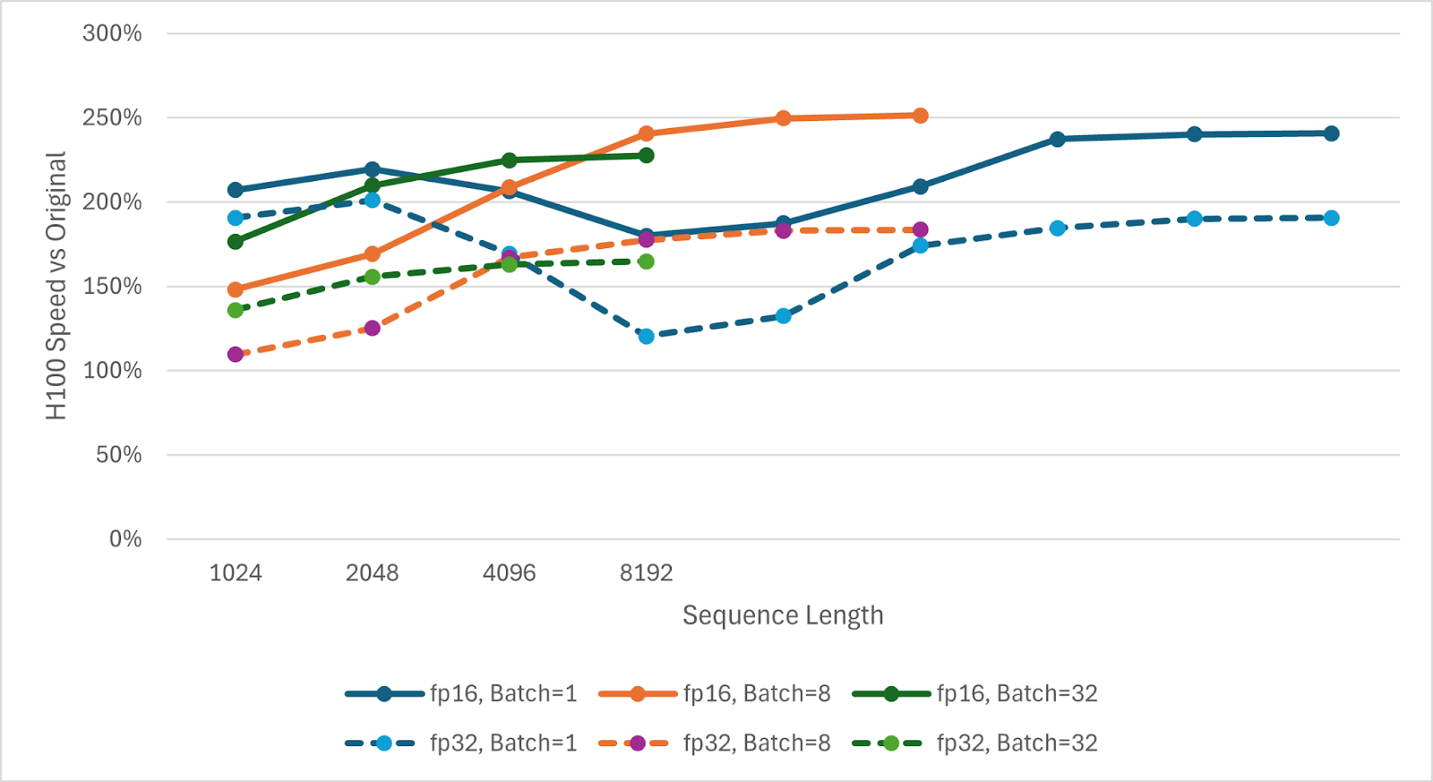
Figure 11. H100 fp32 vs fp16 Accuracy Graph

In Figure 11, we show how our speedup changes when states are in fp32 instead of fp16. Both the fused and original kernels are faster with chunk_size=256 when states are in fp32. This represents a tradeoff of higher compute in return for a smaller state tensor. The fused kernel’s speedup is less for fp32 states than fp16 states, likely because of the different balance of compute and data movement.

Other Architectures

The fused SSD kernel is not limited to Mamba-2. It also applies directly to linear attention, since the SSD formula reduces to the linear attention update when A = 1. In this special case, the fused kernel could be further simplified and optimized for even better performance.

New GPU Features

The fused SSD kernel does not currently use newer GPU features such as the Tensor Memory Accelerator (TMA) and thread block clusters on Hopper GPUs, or the Tensor Memory in Blackwell GPUs. These features can greatly reduce register pressure, which would speed up the SSD and could result in faster Triton configs being possible (e.g., larger block sizes). The thread block clusters could especially be useful for broadcast-loading C, B, and CB matrices that are shared across a group of heads in the SSD kernel. This could give further speedups on new GPUs if necessary.

Further Fusion: Convolution and Layernorm

In this fused SSD kernel, we fused the 5 original SSD kernels. However, the convolution before the SSD and layernorm after the SSD are appealing candidates for fusion because fusing each would remove an entire read and write between kernels. Since the convolution is depth-wise (no channel mixing), the SSD could load d_conv extra along the seqlen dimension and load the conv weights to perform the convolution in registers or shared memory.

We have done some experiments with fusing the layernorm, but with limited benefit. There are two methods to fuse this layernorm:

1. Launch layernorm threadblocks separately. These threadblocks can wait until the corresponding SSD threadblocks have finished and then read the output y from L2 cache instead of VRAM.
2. Sync SSD threadblocks across heads, exchange norm values, and compute the layernorm in registers or shared memory.

Method 2 was very slow because the SSD threadblocks stalled while syncing and had no other work to do while waiting. Method 1 worked, but reading from L2 instead of VRAM doesn’t provide as much benefit as registers/shared memory. So far, the speedup has been far below the theoretical limit, and it’s unclear whether further optimizations would make it worthwhile given the added complexity.

Insights on Model Design

With the optimized fusion of the five SSD kernels, Mamba2 prefill is now even cheaper than before. This shifts the runtime-accuracy tradeoff for Mamba2 layers, which could make scaling up both the size and the number of Mamba2 layers the optimal balance in new LLMs. More design insights include:

• Compute Intensity: The current fused kernel has low compute utilization at the fastest chunk size, so we might be able to afford slightly more complicated operations. Although we could increase compute intensity by increasing the chunk size, that also increases the required registers and other resources, causing an overall slowdown.
• State Precision: In both the fused and original kernels, the State Passing step must be serial instead of parallel. Although sublinear latency parallel scan algorithms exist, in practice, they can be much slower than the serialized version used in Mamba2. Therefore, minimizing the latency of the State Passing computation as a fraction of the total latency is vital to hiding the serialization latency. If the states can be held in low precisions, such as fp16, this significantly helps the fused kernel. Without a fast State Passing step, we might need to split threadblocks more along other dimensions such as headdim, which would slow down the fused kernel overall.
• VRAM vs L2 tradeoff: Since the fused kernel has higher L2 bandwidth utilization than VRAM bandwidth utilization, the cost of sharing less data across threadblocks is less. If an architecture’s performance benefits greatly from smaller groups, the added VRAM reads could have less of a negative impact on performance than it had with the original kernels. On the other hand, new GPU features such as TMA multicast loads could reduce the L2 bandwidth utilization, speeding up the SSD and reducing this imbalance.

vLLM Integration

In order to support variable length sequences with initial states but without padding, vLLM introduces the idea of “pseudo chunks”. Any chunk with tokens for multiple sequences in it has multiple pseudo chunks, one for each sequence in that chunk. Most of the 5 kernels function the same, with State Passing loading initial states when a new sequence starts. However, Chunk Scan has a larger threadblock grid that goes over pseudo chunks instead of chunks. In order to support this in the fused kernel, we have a for loop to process all pseudo chunks in the current chunk. The vLLM Chunk Scan offset its reads and writes based on where the pseudo chunk starts in the real chunk. We use masking based on the sequence index instead, since masking provides a speedup. Both offsetting and masking read/write the same amount of data at runtime, but the masking might be more predictable for the compiler, better aligned, or just simpler. The vLLM fused kernel is still being integrated, but it shows similar speedup.

Conclusion

In summary, we fused the five Triton kernels of the Mamba-2 SSD prefill into one, yielding a 2x speedup for the SSD itself, which translates into a ~8–20% end-to-end inference speedup. This significantly boosts throughput for models using Mamba-2 layers. We are excited to integrate these kernel improvements into open-source projects so that the community can easily leverage faster inference with Mamba-2 based models. Stay tuned for updates as this fused SSD kernel lands in the Mamba codebase and in inference frameworks like vLLM.

Appendix A: Optimization Details

Threadblock Order

The State Passing step causes serialization. For a given head, all but one threadblock stall waiting for the previous chunk to be ready. When our GPU runs about 256-1024 threadblocks concurrently but only one makes progress, we get a significant slowdown. Some of the serialization is hidden by the latency of the Chunk State step since later chunks could still be computing Chunk State rather than being stalled in State Passing, but this is not enough. We have both the nheads and batch dimensions that represent domain parallelism (independent work) in the SSD. Instead of launching threadblocks for a particular batch and head before moving on to the next, we can launch threadblocks for multiple (batch, head) combinations. If we launch n different (batch, head) combinations for the same chunk before moving on to the next chunk, our serialization drops by a factor of n (instead of only 1 threadblock making progress, n threadblocks make progress). This n must be carefully balanced, because if it’s too large, we lose L2 cache locality for passing states, and if it’s too small, threadblocks stall. As a simple heuristic, we launch threadblocks for all nheads before moving on to the next chunk, but finish all chunks before progressing in the batch dimension. For models with much more or less heads or significantly different dimensions, a more complicated threadblock order could involve explicitly combining nheads and batch and then splitting it into an inner and outer dimension, with the inner dimension launching before the next chunk.

Cache Hints

The input and output tensors of operations such as the Mamba2 SSD are typically too large to fit in cache. For example, the input and output for 16k context in a Mamba2 SSD with 128 heads of 64 dim each in fp16 will each consume 16k * 128 * 64 * 2B = 256 MiB. Typical GPU L2 caches are 40-50 MiB. Therefore, some data will be evicted from the L2 cache during that kernel. 

Since most of the output tensor does not fit in the L2 cache, it’s not worth using L2 cache capacity for the output to try to speed up the next operation. We can use a cache hint to indicate that the output tensor has the lowest priority for caches. In general, once we access data for the final time in the kernel, we can mark it as low priority for caches. For often reused data, such as CB (which is shared among heads in a group), we can use a high priority cache hint to reduce the chance of eviction.

We can also avoid flushing L1 cache during some sync atomics by specifying “release” semantics. This tells the compiler that previously written data must be globally visible before the atomic operation (e.g. if we are setting a “ready” flag), but this thread does not need to invalidate any caches.

Conditional Separation

In the State Passing step, we have two special cases: reading the initial state instead of the previous chunk’s global state and writing to the final state instead of to the global states tensor. Although conceptually these special cases should only involve swapping the base pointer to read/write to, the initial and final state conditionals increase register pressure and slow down the fused kernel. To solve this, we can handle the special cases outside of the fused SSD kernel. If we replace the nchunks dimension in our state tensor with nchunks + 1, we can copy the initial states into the 0th chunk and copy out final states from the last chunk. These copies are done using the pytorch sliced assignment syntax, which results in small kernels with negligible runtime or launch overhead.

Intermediate Datatypes

For some computations, such as applying the A decay to B in Chunk Scan, we can use fp16 for the computation instead of fp32. This also swaps upcasting B and downcasting the result with only downcasting the scale, reducing casting instructions.

Compile-Time Masks

Triton requires that the dimensions of blocks of tensors in a threadblock are powers of 2 known at compile time. This forces all stores and loads to operate on power-of-2 blocks that might not divide the target tensor exactly. We therefore use masks to cover the entire tensor but avoid reading or writing out of bounds data (or the next block of data). These masks are the same dimensions as the tensor block. However, these masks are not always necessary because model dimensions like headdim are often divisible by the block size and do not change between different inputs. Triton supports tl.constexpr compile-time parameters and setting them based on other parameters with @triton.heuristics. Therefore, we can automatically enable or disable the headdim dimension of the mask at runtime based on if the headdim is divisible by the block size. Although this occurs at “runtime”, it really only occurs once during the initial JIT compilation of the kernel for this model.

Chunk Size

The Mamba2 SSD algorithm takes asymptotically constant computation per token (computation scales linearly with sequence length), but it has a base case of some chunk size that is computed quadratically. Between chunks, the linear algorithm is used, but within a chunk, the quadratic algorithm is used. For more details, see https://tridao.me/blog/2024/mamba2-part1-model/#state-space-duality.

The optimal chunk size represents a tradeoff of higher computation and resources required vs higher hardware utilization and less intermediate states. With the original unfused kernels, the optimal chunk size for Mamba2-2.7B had been 256. However, with the new fused kernel, the optimal chunk size is now 128 for the same model. This smaller chunk size also has the added benefit of reducing register pressure, making the kernel less sensitive to small changes like enabling masks or using higher precision for intermediate results.

Currently, the convention for Mamba2 models is to specify the chunk size in the model’s config. However, since the optimal chunk size varies depending on the original vs fused kernels, it could be better to use a heuristic or autotune the chunk size. This might not be straightforward since the code surrounding the SSD kernels might assume a particular chunk size.

Scale Multiplication Operand

For Chunk State, we can equivalently apply the A decay to X instead of B, since the dimension to be scaled is the inner dimension of the matmul of X and B. Essentially, we do (X * A[None, :]) @ B instead of (X @ (A[:, None] * B). This is faster, probably due to a more similar layout causing less register data movement. For example, due to the required Tensor Core data layout, each thread might already have the required A values to multiply with its X values, but to scale B, we might have to load in a different layout and shuffle data back to the required Tensor Core layout.

Appendix B: Summary of Stall Reasons

If we look at the source in NVIDIA Nsight Compute, we can see the warp stalls for each line of code and assembly instruction in the fused kernel on an H100. Assuming that the kernel and block sizes are optimal, warp stalls can reveal potential areas for optimization.

1. In order to ensure correctness, we use an atomic add to get threadblock ids in increasing order. This accounts for about 3% of the total warp stalls.
2. Both the Chunk Cumsum and BMM parts of the fused kernel are very fast, so they only cause less than 2% of warp stalls each.
3. Atomically checking that the Chunk Cumsum and BMM threadblocks have prepared data for this Chunk State threadblock accounts for about 1.5% of warp stalls.
4. Chunk State has about 12% of total warp stalls in loading dA, X, and especially B. It also has about 7% stalls in barriers related to scaling and using Tensor Cores.
5. Despite being serialized along chunks, State Passing has less than 3% stalls on synchronization (including awaiting the previous chunk). Loading the previous states does not cause significant stalling, but updating the state and storing cause about 6% stalls awaiting shared memory or a barrier.
6. For the previous state’s contribution in Chunk Scan, loading C is about 5% loading stalls, prev_states is about 3% barrier stalls, and the computation is about 8% barrier, loading (for scale), and instruction dependency stalls.
7. The current chunk’s contribution in Chunk Scan has about 13% stalls in loading data and 18% stalls in computation (including scaling).
8. The residual (scaled by D) accounts for about 6% of total stalls for loading, shared memory, and computation.

Overall, these stalls are for legitimate reasons and are not easy to optimize away.