1.0 Summary
We present an optimized Triton FP8 GEMM (General Matrix-Matrix Multiply) kernel TK-GEMM, which leverages SplitK parallelization. For small batch size inference, TK-GEMM delivers up to 1.94x over the base Triton matmul implementation, 1.87x speedup over cuBLAS FP8 and 1.71x over cuBLAS FP16 for Llama3-70B inference problem sizes on NVIDIA H100 GPUs.
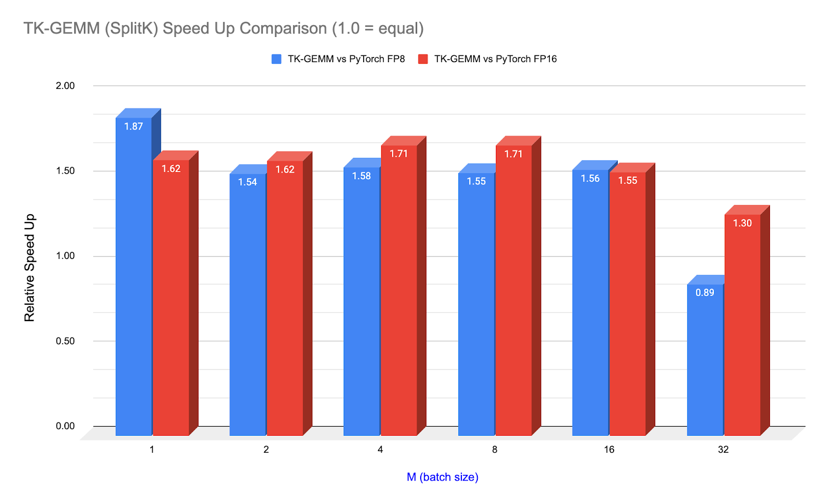
Figure 1. TK-GEMM Speedup over PyTorch (calling cuBLAS) for Llama3-70B Attention Layer Matrix Shapes (N=K=8192)
In this blog, we will cover how we designed an optimized kernel using Triton for FP8 inference and tuned it for Lama3-70B inference. We will cover FP8 (8-bit floating point), a new datatype supported by Hopper generation GPUs (SM90), the key SM90 features that Triton supports, and how we modified the parallelization to be able to maximize memory throughput for memory-bound (inference) problem sizes.
We also dedicate a section on CUDA graphs, an important technology that will help materialize kernel level speedups and enable developers who want to use Triton kernels in production settings to get additional performance gain.
Repo and code available at: https://github.com/pytorch-labs/applied-ai
2.0 FP8 Datatype
The FP8 datatype was introduced jointly by Nvidia, Arm and Intel and serves as a successor to 16-bit floating point types. With half the bit count, it has the potential to provide significant throughput improvements over its predecessors for Transformer networks. The FP8 datatype consists of 2 formats:
E4M3 (4-bit exponent and 3-bit mantissa). Able to store +/ 448 and nan.
E5M2 (5-bit exponent and 2-bit mantissa). Able to store +/- 57,334, nan and inf.
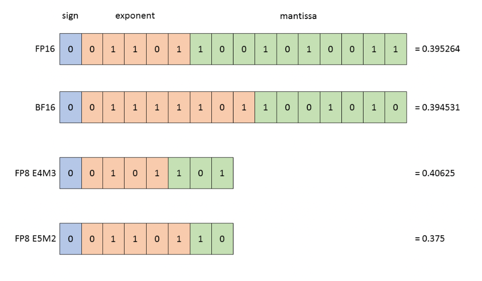
Above: BF16, FP16, FP8 E4M3 and FP8 E5M2.
To show precision differences, the closest representation to 0.3952 is shown in each format.
Image Credit: Nvidia
We use E4M3 in inference and forward pass training due its higher precision and E5M2 in training backward pass due to its higher dynamic range. Nvidia has designed their H100 FP8 Tensor Core to provide a peak of 3958 TFLOPS, 2x the FLOPS of the FP16 Tensor Core.
We designed our Triton kernel with these hardware innovations in mind and in the rest of the blog we will discuss methods to leverage and verify that these features are indeed being utilized by the Triton compiler.
3.0 Triton Hopper Support and FP8 Tensor Core Instruction
The Hopper GPU architecture has added the following new features that we can expect will accelerate FP8 GEMM.
- TMA (Tensor Memory Accelerator) Hardware Unit
- WGMMA (Warp Group Matrix Multiply-Accumulate Instruction)
- Threadblock Clusters
Triton currently takes advantage of one of these features, the wgmma instruction, whereas PyTorch (calling cuBLAS) leverages all 3 which makes these speedups even more impressive. To fully take advantage of the Hopper FP8 Tensor Core, the wgmma is necessary even though the older mma.sync instruction is still supported.
The key difference between the mma and wgmma instructions is that instead of 1 CUDA warp being responsible for an output shard, an entire warp group, 4 CUDA warps, asynchronously contributes to an output shard.
To see what this instruction looks like in practice, and to verify that our Triton Kernel is indeed utilizing this feature we analyzed the PTX and SASS assembly using nsight compute.
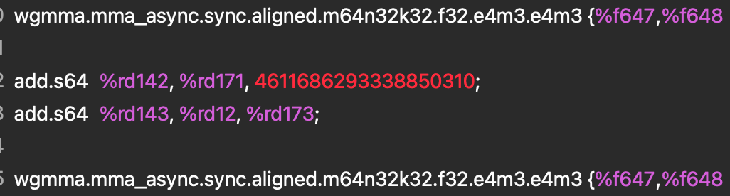
Figure 2. PTX Assembly
This instruction is further lowered into a QGMMA instruction in SASS.
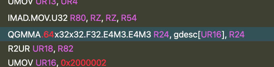
Figure 3. SASS Assembly
Both instructions tell us that we are multiplying two FP8 E4M3 input tensors and accumulating in F32, which confirms that the TK-GEMM Kernel is utilizing the FP8 Tensor Core and the lowering is being done correctly.
4.0 SplitK Work Decomposition
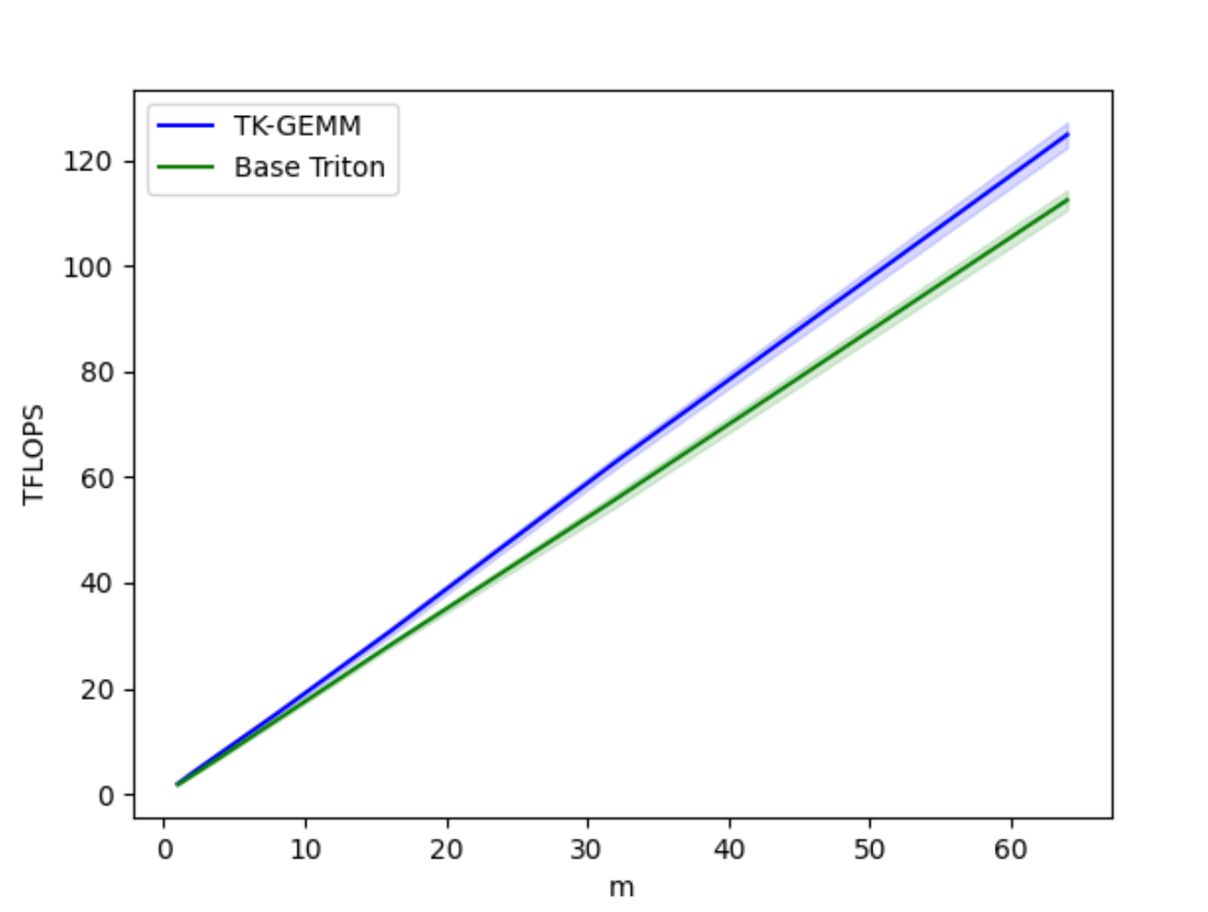
Figure 4. TK-GEMM vs Base Triton GEMM TFLOPS for M = 1-64
The base Triton FP8 GEMM implementation does not perform well for the small M regime, where for a matrix multiplication of A (MxN) x B (NxK), M < N, K. To optimize for this type matrix profile we applied a SplitK work decomposition instead of the Data Parallel decomposition found in the base Triton kernel. This greatly improved latencies for the small M regime.
For background, SplitK launches additional thread blocks along the k dimension to calculate partial output sums. The partial results from each thread block are then summed using an atomic reduction. This allows for finer grained work decomposition with resultant performance improvements. More details on SplitK are available in our arxiv paper.
After carefully tuning the other relevant hyperparameters for our kernel such as tile sizes, number of warps and the number of pipeline stages to Llama3-70B problem sizes we were able to produce up to 1.94x speedup over the Triton base implementation. For a more comprehensive introduction to hyperparameter tuning, see our blog.
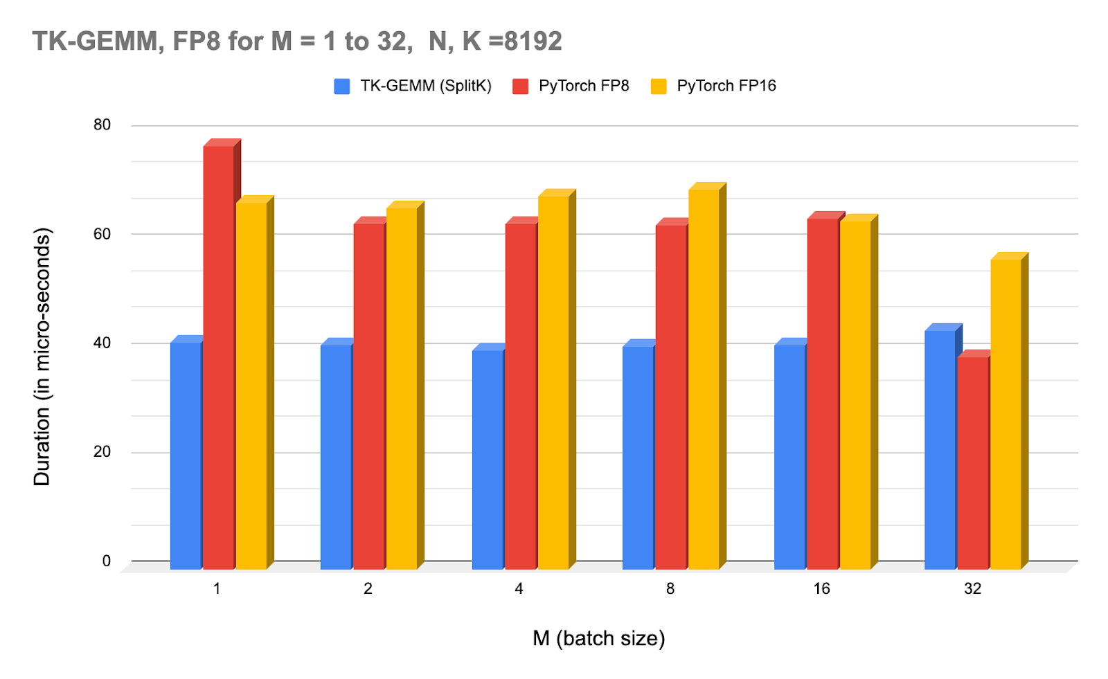
Above: NCU profiler times for TK-GEMM under varying batch sizes, and compared with PyTorch (calling cuBLAS) FP8 and FP16.
Note that starting at M=32, the cuBLAS FP8 kernel starts to outperform TK-GEMM. For M >= 32, we suspect that hyperparameters we found are not optimal, and thus another set of experiments is required to determine the optimal parameters for the mid-sized M regime.
5.0 CUDA Graphs to Enable End-to-End Speedup
To be able to realize these speedups in an end-to-end setting, we must take into account both the kernel execution time (GPU duration) as well as the wall time (CPU+GPU) duration. Triton kernels, which are handwritten (as opposed to torch compile generated) are known to suffer from high-kernel launch latencies. If we use torch profiler to trace the TK-GEMM kernel we can see the call stack on the CPU side to pinpoint exactly what is causing the slowdown.
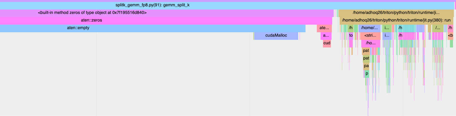
Figure 5. CPU Launch Overhead: 2.413ms
From above, we see that the majority of the wall time of our optimized kernel is dominated by JIT (Just-in-Time) compilation overhead. To combat this we can use CUDA graphs.
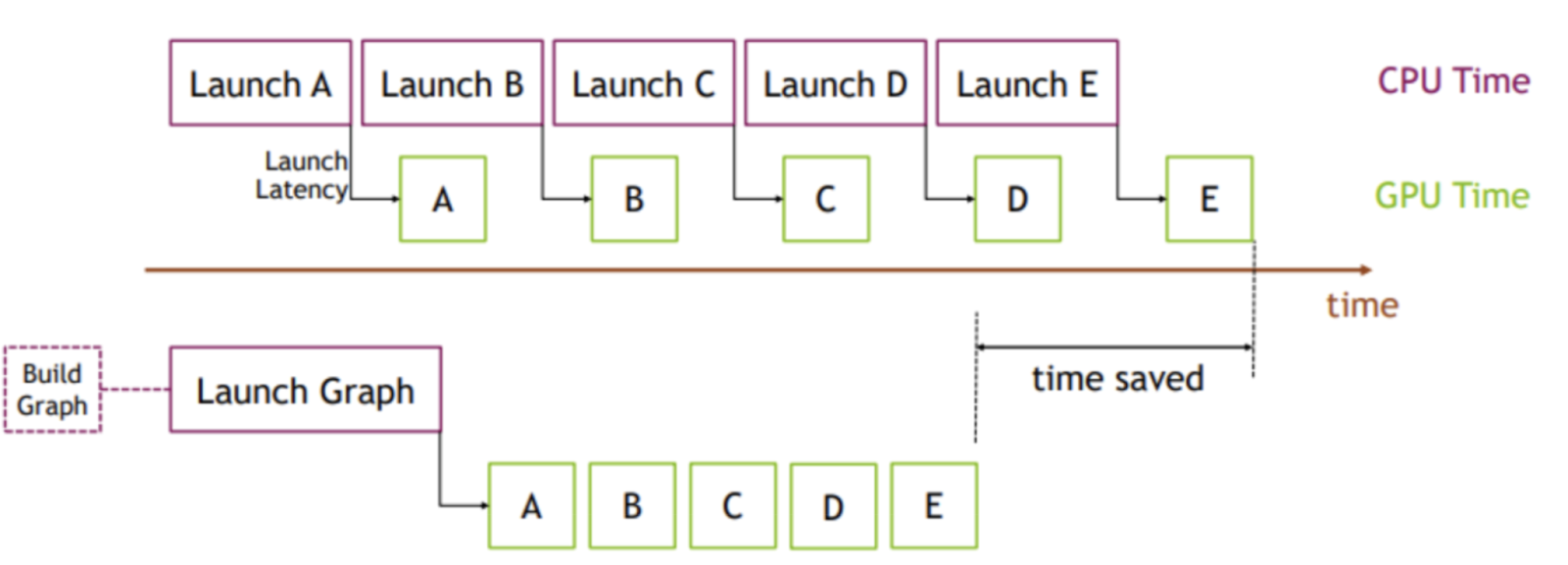
Figure 6. CUDA Graphs Visualization
Image Credit: PyTorch
The key idea is instead of multiple kernel launches, we instead can create and instantiate a graph (1 time cost) and then submit that instance of the graph for execution. To illustrate this point we simulate a Llama3-70B Attention layer, As shown in the below figure generated using nsight systems, the time between each GEMM is 165us compared to the 12us spent on the actual matmul due the CPU kernel launch overhead. This means that 92% of the time of the time in an Attention layer the GPU is idle and not doing any work.
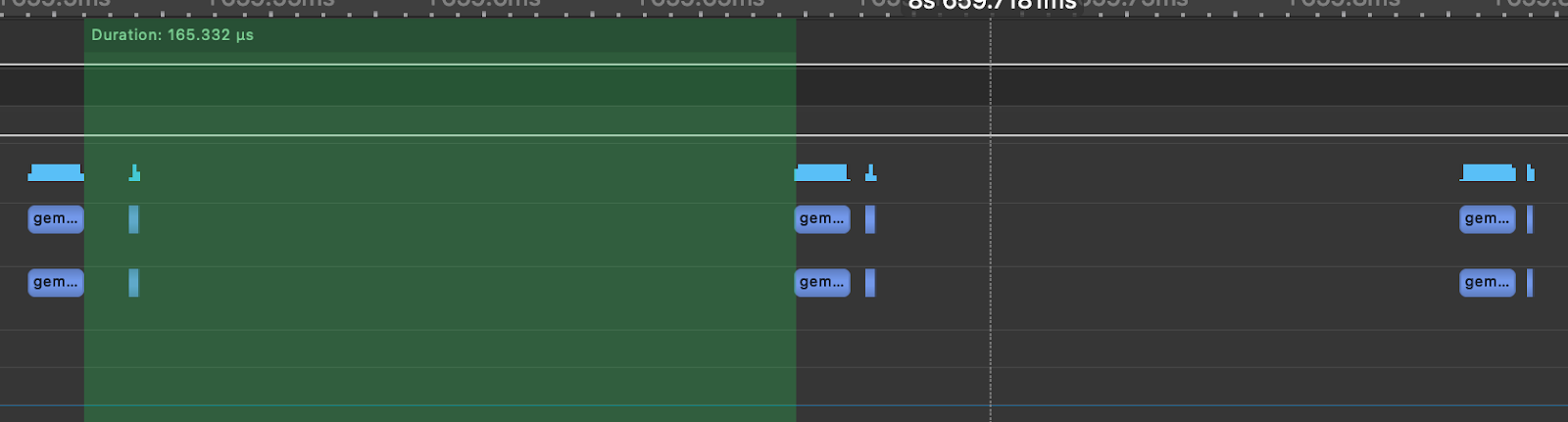
Figure 7. Simulated Llama3-70B Attention Layer with TK-GEMM
To show the impact of CUDA graphs, we then created a graph of the TK-GEMM kernel in the toy Attention layer and replayed the graph. Below, we can see that the gaps between kernel executions are reduced to 6.65us.
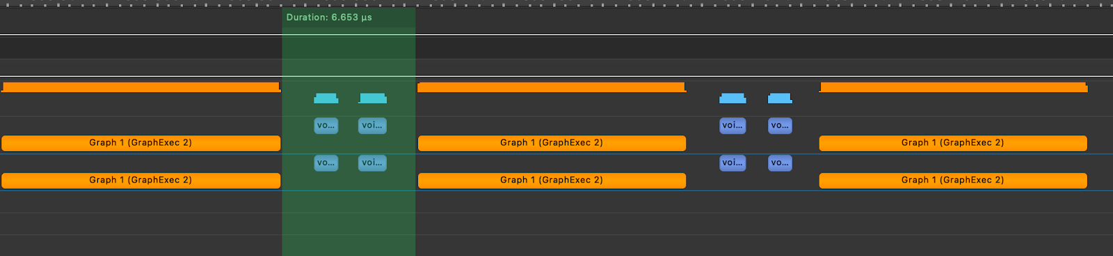
Figure 8. Simulated Llama3-70B Attention Layer with TK-GEMM and CUDA Graphs
In practice, this optimization would result in a 6.4x speedup of a single attention layer in Llama3-70B, over naively using TK-GEMM in a model without CUDA graphs.
6.0 Potential Future Optimization Paths
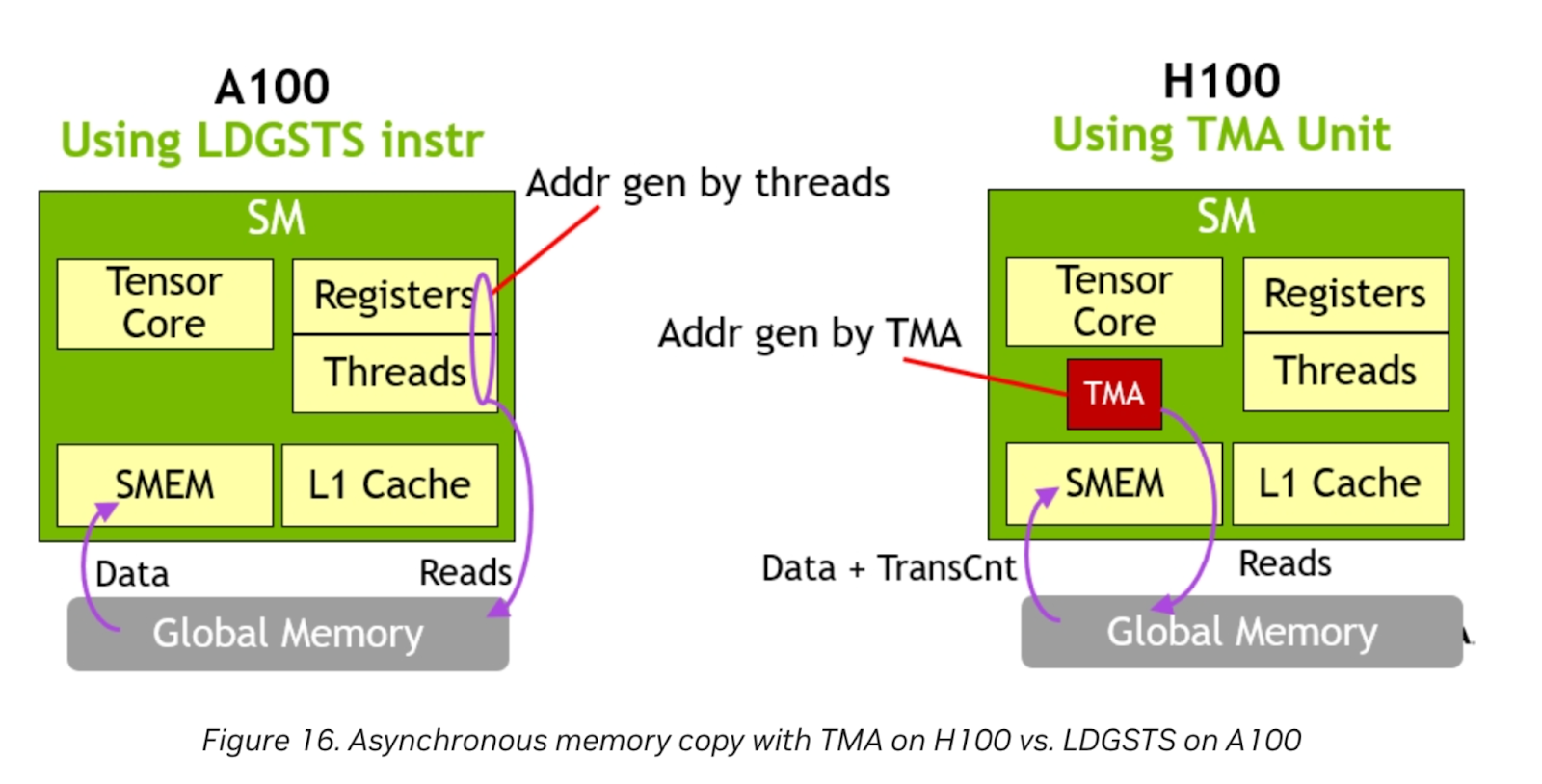
Figure 9. TMA Hardware Unit
Image Credit: Nvidia
The Nvidia H100 features a TMA hardware unit. The dedicated TMA unit frees up registers and threads to do other work, as address generation is completely handled by the TMA. For memory bound problem sizes, this can provide even further gain when Triton enables support for this feature.
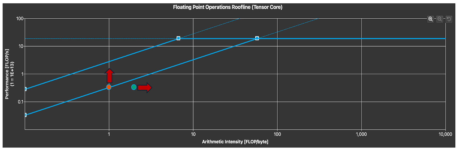
Figure 10. Tensor Core Utilization (Arrows Indicate Degrees of Freedom)
To identify how well we are utilizing the Tensor Core, we can analyze the roofline chart. Notice that we are in the memory-bound region as expected for small M. To improve kernel latency we can either increase the arithmetic intensity, which with a fixed problem size can only be achieved through exploiting data locality and other loop optimizations or increasing the memory throughput. This requires either a more optimal parallel algorithm specialized for the FP8 datatype as well as the type of problem size characteristics we expect to see in FP8 inference.
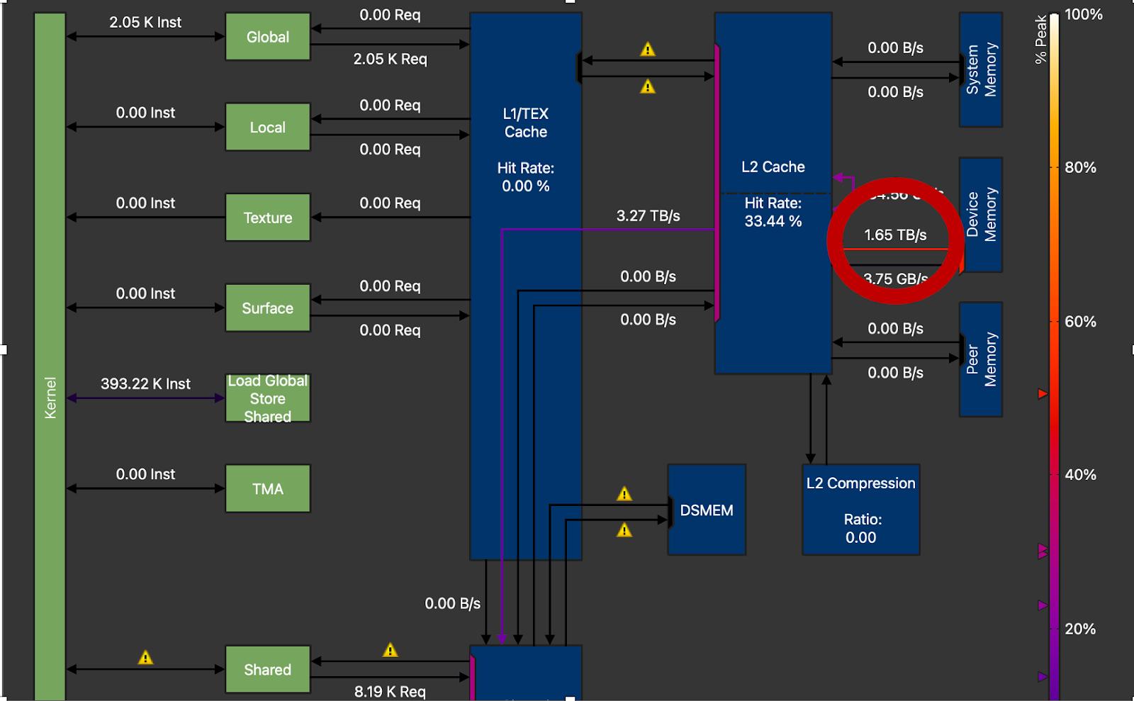
Figure 11. DRAM Throughput Circled, 1.65TB/s vs Peak 3.35TB/s on H100 (M=16, N=8192, K=8192)
Lastly, we can see that we are only achieving around 50% of peak DRAM throughput on the NVIDIA H100. High performance GEMM kernels typically achieve around 70-80% of peak throughput. This means that there is still a lot of room to improve and the techniques mentioned above (loop unrolling, optimized parallelization) are needed for additional gain.
7.0 Future Work
For future research, we would like to explore CUTLASS 3.x and CuTe to leverage more direct control over Hopper features especially in terms of obtaining direct TMA control and exploring pingpong architectures, which have shown promising results for FP8 GEMM.