This post is the second part of a multi-series blog focused on how to accelerate generative AI models with pure, native PyTorch. We are excited to share a breadth of newly released PyTorch performance features alongside practical examples to see how far we can push PyTorch native performance. In part one, we showed how to accelerate Segment Anything over 8x using only pure, native PyTorch. In this blog we’ll focus on LLM optimization.
Over the past year, generative AI use cases have exploded in popularity. Text generation has been one particularly popular area, with lots of innovation among open-source projects such as llama.cpp, vLLM, and MLC-LLM.
While these projects are performant, they often come with tradeoffs in ease of use, such as requiring model conversion to specific formats or building and shipping new dependencies. This begs the question: how fast can we run transformer inference with only pure, native PyTorch?
As announced during our recent PyTorch Developer Conference, the PyTorch team wrote a from-scratch LLM almost 10x faster than baseline, with no loss of accuracy, all using native PyTorch optimizations. We leverage a breadth of optimizations including:
- Torch.compile: A compiler for PyTorch models
- GPU quantization: Accelerate models with reduced precision operations
- Speculative Decoding: Accelerate LLMs using a small “draft” model to predict large “target” model’s output
- Tensor Parallelism: Accelerate models by running them across multiple devices.
And, even better, we can do it in less than 1000 lines of native PyTorch code.
If this excites you enough to jump straight into the code, check it out at https://github.com/pytorch-labs/gpt-fast!
Note: We will be focusing on latency (i.e. batch size=1) for all of these benchmarks. Unless otherwise specified, all benchmarks are run on an A100-80GB, power limited to 330W.
Starting Point (25.5 tok/s)
Let’s start off with an extremely basic and simple implementation.
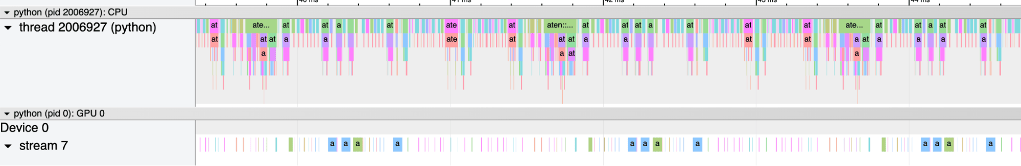
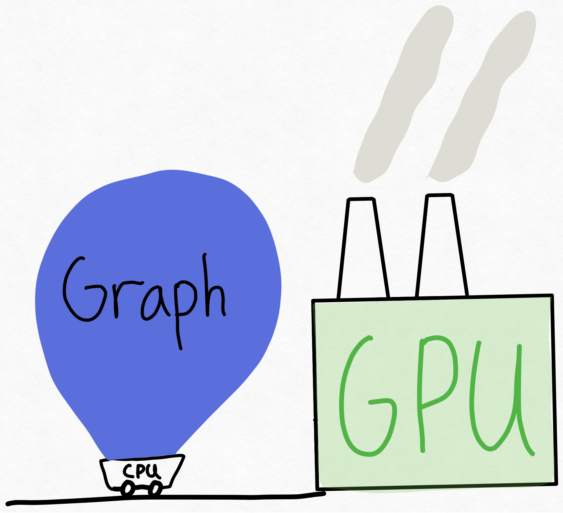
Sadly, this does not perform very well. But why? Looking at a trace reveals the answer – it’s heavily CPU overhead bound! What this means is that our CPU is not able to tell the GPU what to do fast enough for the GPU to be fully utilized.
Imagine the GPU as this super massive factory with a ridiculous amount of compute available. Then, imagine the CPU as some messenger shuttling instructions back and forth to the GPU. Remember, in large scale deep learning systems, the GPU is responsible for doing 100% of the work! In such systems, the only role of the CPU is to tell the GPU what work it should be doing.
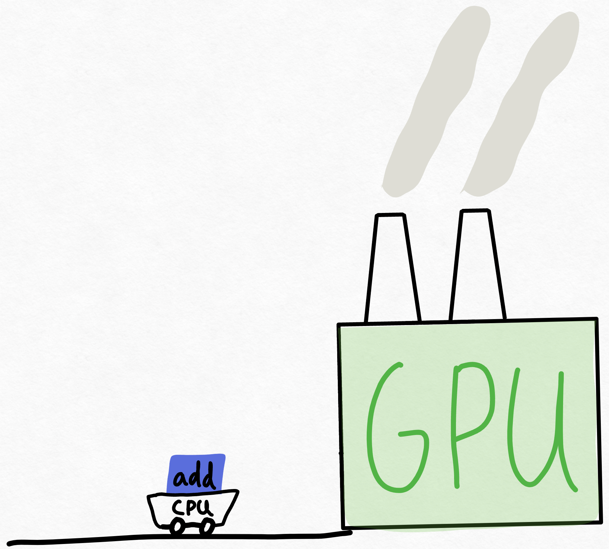
So, the CPU runs over and tells the GPU to do an “add”, but by the time the CPU can give the GPU another chunk of work, the GPU has long finished the previous chunk of work.
Despite the fact that the GPU needs to perform thousands of computations while the CPU only needs to do orchestration work, this is surprisingly common! There’s a variety of reasons for this, ranging from the fact that the CPU is likely running some single-threaded Python to the fact that GPUs are just incredibly fast nowadays.
Regardless of the reason, we now find ourselves in the overhead-bound regime. So, what can we do? One, we could rewrite our implementation in C++, perhaps even eschew frameworks entirely and write raw CUDA. Or…. we could just send more work to the GPU at once.
By just sending a massive chunk of work at once, we can keep our GPU busy! Although during training, this may just be accomplished by increasing your batch size, how do we do this during inference?
Enter torch.compile.
Step 1: Reducing CPU overhead through torch.compile and a static kv-cache (107.0 tok/s)
Torch.compile allows us to capture a larger region into a single compiled region, and particularly when run with mode=”reduce-overhead”, is very effective at reducing CPU overhead. Here, we also specify fullgraph=True, which validates that there are no “graph breaks” in your model (i.e. portions that torch.compile cannot compile). In other words, it ensures that torch.compile is running to its fullest potential.
To apply it, we simply wrap a function (or a module) with it.
torch.compile(decode_one_token, mode="reduce-overhead", fullgraph=True)
However, there are a couple of nuances here that make it somewhat nontrivial for folks to get significant performance boosts from applying torch.compile to text generation.
The first obstacle is the kv-cache. The kv-cache is an inference-time optimization that caches the activations computed for the previous tokens (see here for a more in-depth explanation). However, as we generate more tokens, the “logical length” of the kv-cache grows. This is problematic for two reasons. One is that reallocating (and copying!) the kv-cache every time the cache grows is simply expensive. The other one is that this dynamism makes it harder to reduce the overhead, as we are no longer able to leverage approaches like cudagraphs.
To resolve this, we use a “static” kv-cache, which means that we statically allocate the maximum size of the kv-cache, and then mask out the unused values in the attention portion of the computation.

The second obstacle is the prefill phase. Transformer text generation is best thought of as a two phase process: 1. The prefill where the entire prompt is processed, and 2. Decoding where each token is generated autoregressively.
Although decoding can be made entirely static once the kv-cache is made static, the prefill stage still requires significantly more dynamism, due to having a variable prompt length. Thus, we actually need to compile the two stages with separate compilation strategies.

Although these details are a bit tricky, the actual implementation is not very difficult at all (see gpt-fast)! And the performance boost is dramatic.
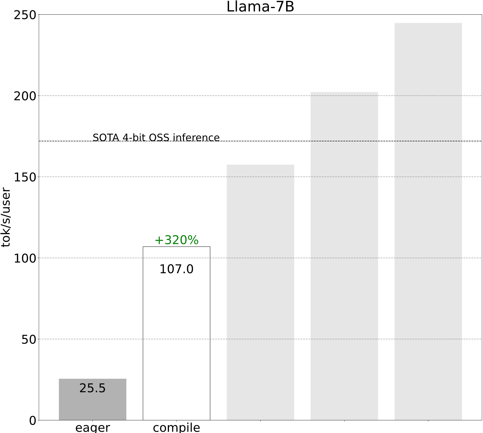
All of a sudden, our performance improves by more than 4x! Such performance gains are often common when one’s workload is overhead bound.
Sidenote: How is torch.compile helping?
It is worth disentangling how exactly torch.compile is improving performance. There’s 2 main factors leading to torch.compile’s performance.
The first factor, like mentioned above, is overhead reduction. Torch.compile is able to reduce overhead through a variety of optimizations, but one of the most effective ones is called CUDAGraphs. Although torch.compile applies this automatically for you when “reduce-overhead” is set, saving the extra work and code you need to write when doing this yourself manually without torch.compile.
The second factor, however, is that torch.compile simply generates faster kernels. In the decoding benchmark above, torch.compile actually generates every single kernel from scratch, including both the matrix multiplications and the attention! And even cooler, these kernels are actually faster than the built in alternatives (CuBLAS and FlashAttention2)!
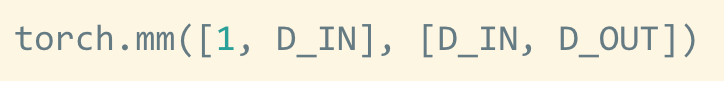
This may sound implausible to many of you, considering how hard it is to write efficient matrix multiplication/attention kernels, and how much manpower has been put into CuBLAS and FlashAttention. The key here, however, is that transformer decoding has very unusual computational properties. In particular, because of the KV-cache, for BS=1 every single matrix multiplication in a transformer is actually a matrix vector multiplication.
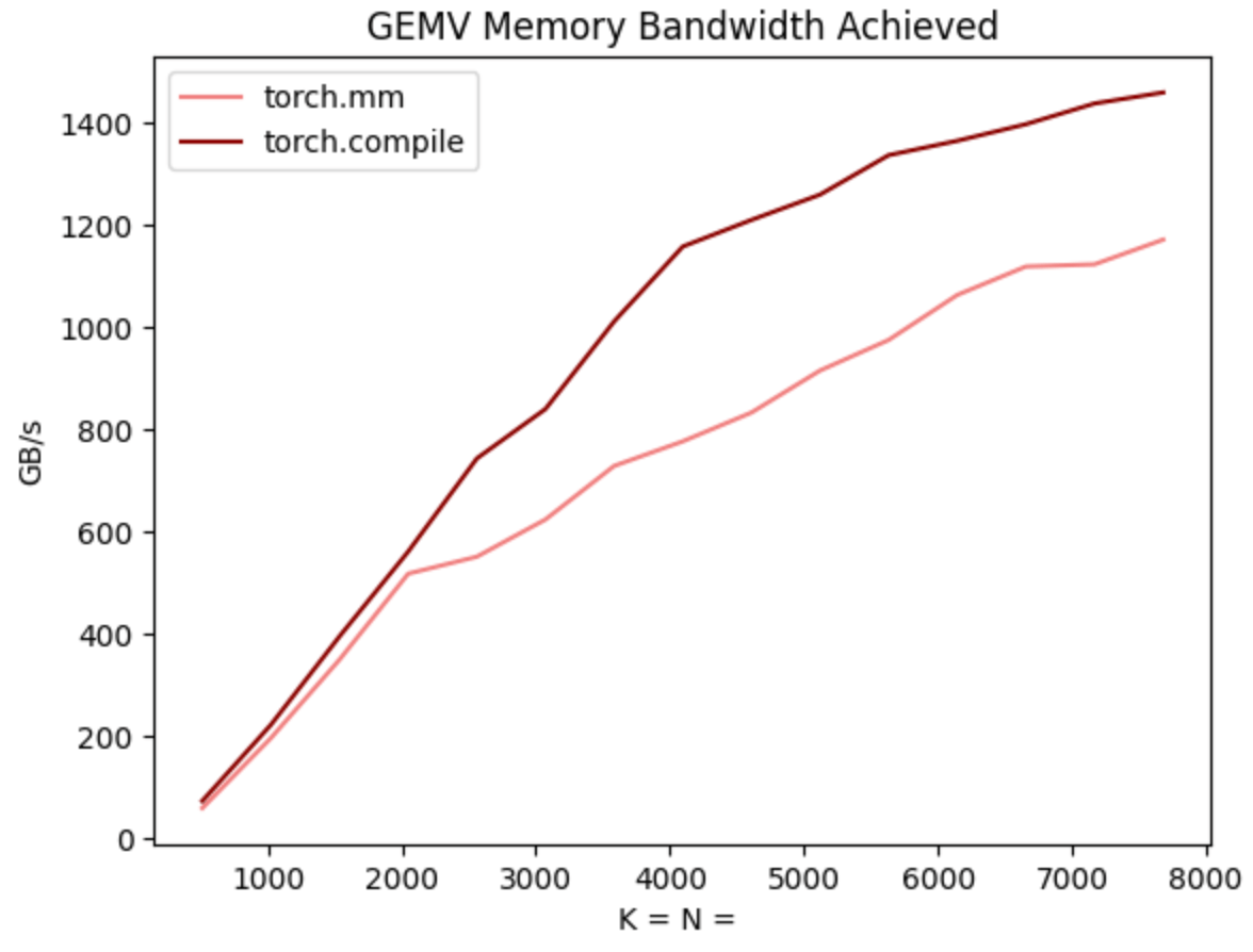
This means that the computations are completely memory-bandwidth bound, and as such, are well within the range of compilers to automatically generate. And in fact, when we benchmark torch.compile’s matrix-vector multiplications against CuBLAS, we find that torch.compile’s kernels are actually quite a bit faster!
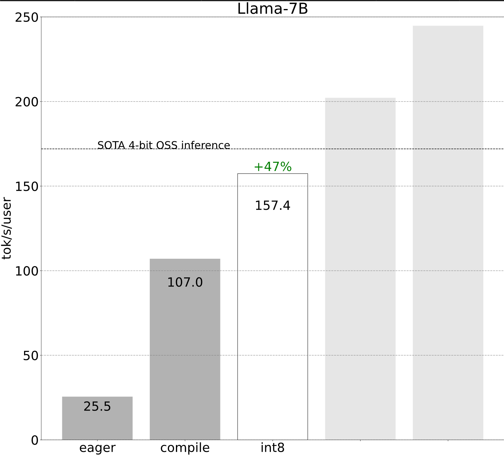
Step 2: Alleviating memory bandwidth bottleneck through int8 weight-only quantization (157.4 tok/s)
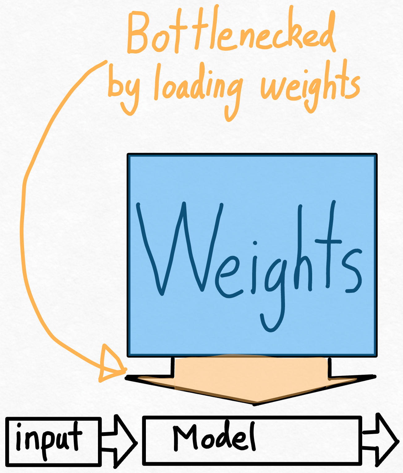
So, given that we’ve already seen massive speedups from applying torch.compile, is it possible to do even better? One way to think about this problem is to compute how close we are to the theoretical peak. In this case, the largest bottleneck is the cost of loading the weights from GPU global memory to registers. In other words, each forward pass requires us to “touch” every single parameter on the GPU. So, how fast can we theoretically “touch” every single parameter in a model?
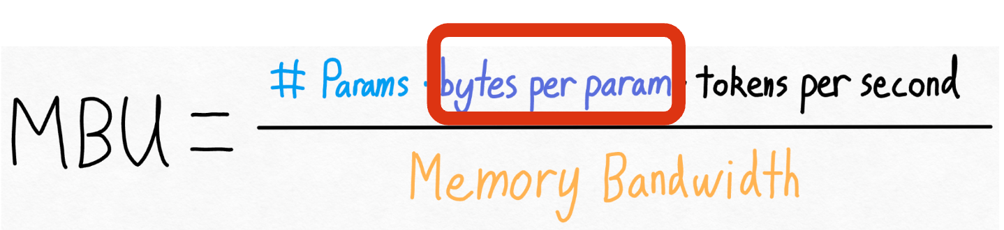
To measure this, we can use Model Bandwidth Utilization (MBU). This measures what percentage of our memory bandwidth we’re able to use during inference.
Computing it is pretty simple. We simply take the total size of our model (# params * bytes per param) and multiply it by the number of inferences we can do per second. Then, we divide this by the peak bandwidth of the GPU to get our MBU.

For example, for our above case, we have a 7B parameter model. Each parameter is stored in fp16 (2 bytes per parameter), and we achieved 107 tokens/s. Finally, our A100-80GB has a theoretical 2 TB/s of memory bandwidth.

Putting this all together, we get **72% MBU! **This is quite good, considering that even just copying memory struggles to break 85%.
But… it does mean that we’re pretty close to the theoretical limit here, and that we’re clearly bottlenecked on just loading our weights from memory. It doesn’t matter what we do – without changing the problem statement in some manner, we might only be able to eek out another 10% in performance.
Let’s take another look at the above equation. We can’t really change the number of parameters in our model. We can’t really change the memory bandwidth of our GPU (well, without paying more money). But, we can change how many bytes each parameter is stored in!
Thus, we arrive at our next technique – int8 quantization. The idea here is simple. If loading our weights from memory is our main bottleneck, why don’t we just make the weights smaller?
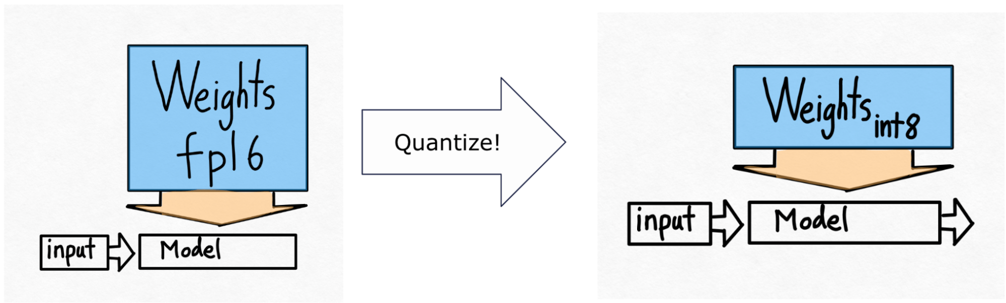
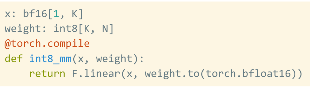
Note that this is quantizing only the weights – the computation itself is still done in bf16. This makes this form of quantization easy to apply with very little to no accuracy degradation.
Moreover, torch.compile can also easily generate efficient code for int8 quantization. Let’s look again at the above benchmark, this time with int8 weight-only quantization included.
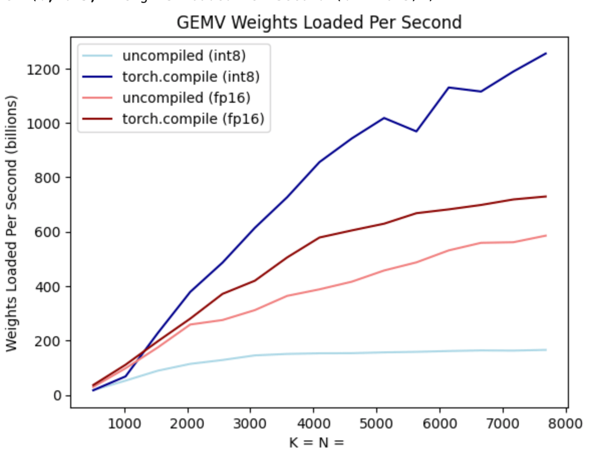
As you can see from the dark blue line (torch.compile + int8), there is a significant performance improvement when using torch.compile + int8 weight-only quantization! Moreover, the light-blue line (no torch.compile + int8) is actually much worse than even the fp16 performance! This is because in order to take advantage of the perf benefits of int8 quantization, we need the kernels to be fused. This shows one of the benefits of torch.compile – these kernels can be automatically generated for the user!
Applying int8 quantization to our model, we see a nice 50% performance improvement, bringing us up to 157.4 tokens/s!
Step 3: Reframing the problem using speculative decoding
Even after using techniques like quantization, we’re still faced with another problem. In order to generate 100 tokens, we must load our weights 100 times.
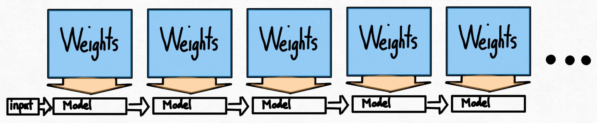
Even if the weights are quantized, we still must load our weights over and over, once for each token we generate! Is there any way around this?
At first glance, the answer might seem like no – there’s a strict serial dependency in our autoregressive generation. However, as it turns out, by utilizing speculative decoding, we’re able to break this strict serial dependency and obtain speedups!
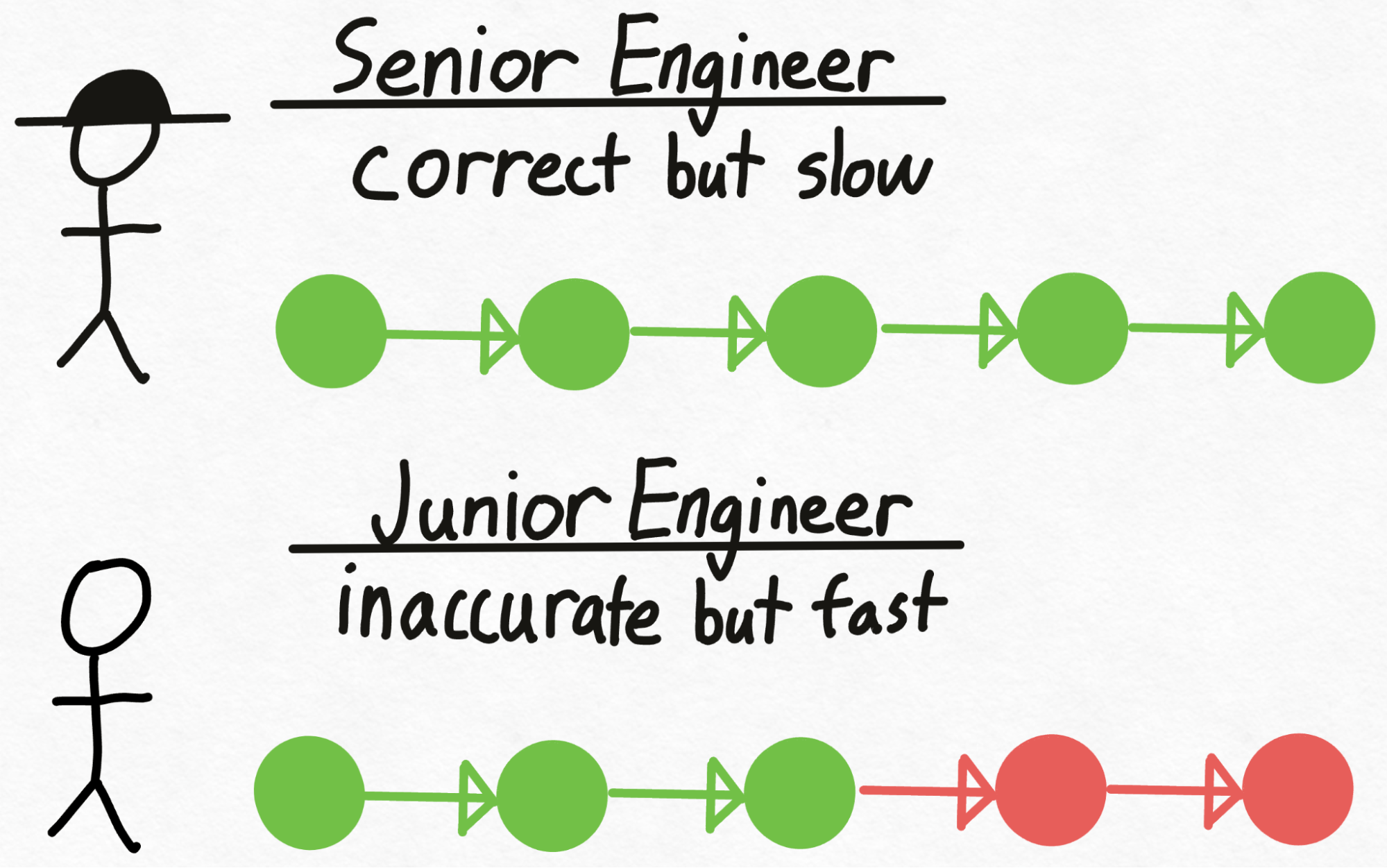
Imagine you had a senior engineer (called Verity), who makes the right technical decisions but is rather slow at writing code. However, you also have a junior engineer (called Drake), who doesn’t always make the right technical decisions but can write code much faster (and cheaper!) than Verity. How can we take advantage of Drake (the junior engineer) to write code faster while ensuring that we are still making the right technical decisions?

First, Drake goes through the labor-intensive process of writing the code, making technical decisions along the way. Next, we give the code to Verity to review.
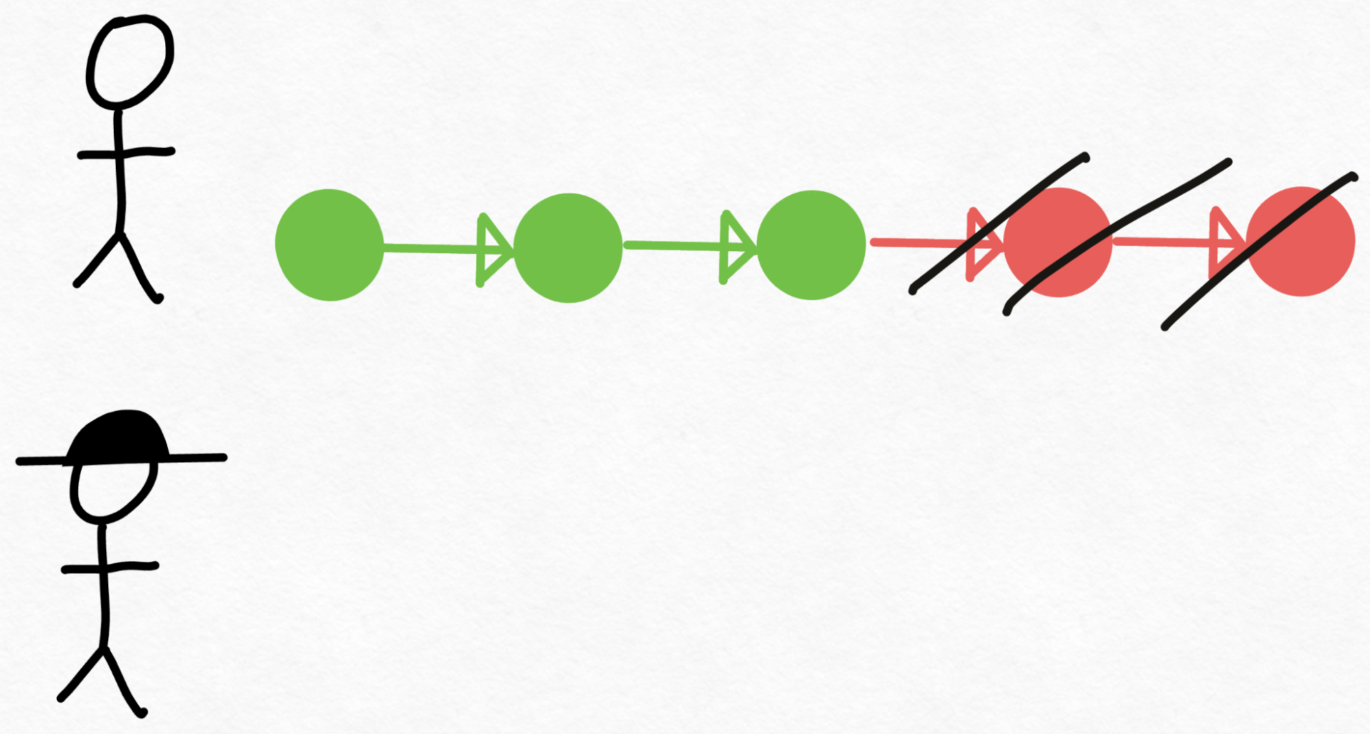
Upon reviewing the code, Verity might decide that the first 3 technical decisions Drake made are correct, but the last 2 need to be redone. So, Drake goes back, throws away his last 2 decisions, and restarts coding from there.
Notably, although Verity (the senior engineer) has only looked at the code once, we are able to generate 3 pieces of validated code identical to what she would have written! Thus, assuming Verity is able to review the code faster than it would have taken her to write those 3 pieces herself, this approach comes out ahead.
In the context of transformer inference, Verity would be played by the role of the larger model whose outputs we want for our task, called the verifier model. Similarly, Drake would be played by a smaller model that’s able to generate text much faster than the larger model, called the draft model. So, we would generate 8 tokens using the draft model, and then process all eight tokens in parallel using the verifier model, throwing out the ones that don’t match.
Like mentioned above, one crucial property of speculative decoding is that it does not change the quality of the output. As long as the time it takes for generating the tokens using the draft model + verifying the tokens is less than it would have taken to generate those tokens, we come out ahead.
One of the great things about doing this all in native PyTorch is that this technique is actually really easy to implement! Here’s the entirety of the implementation, in about 50 lines of native PyTorch.
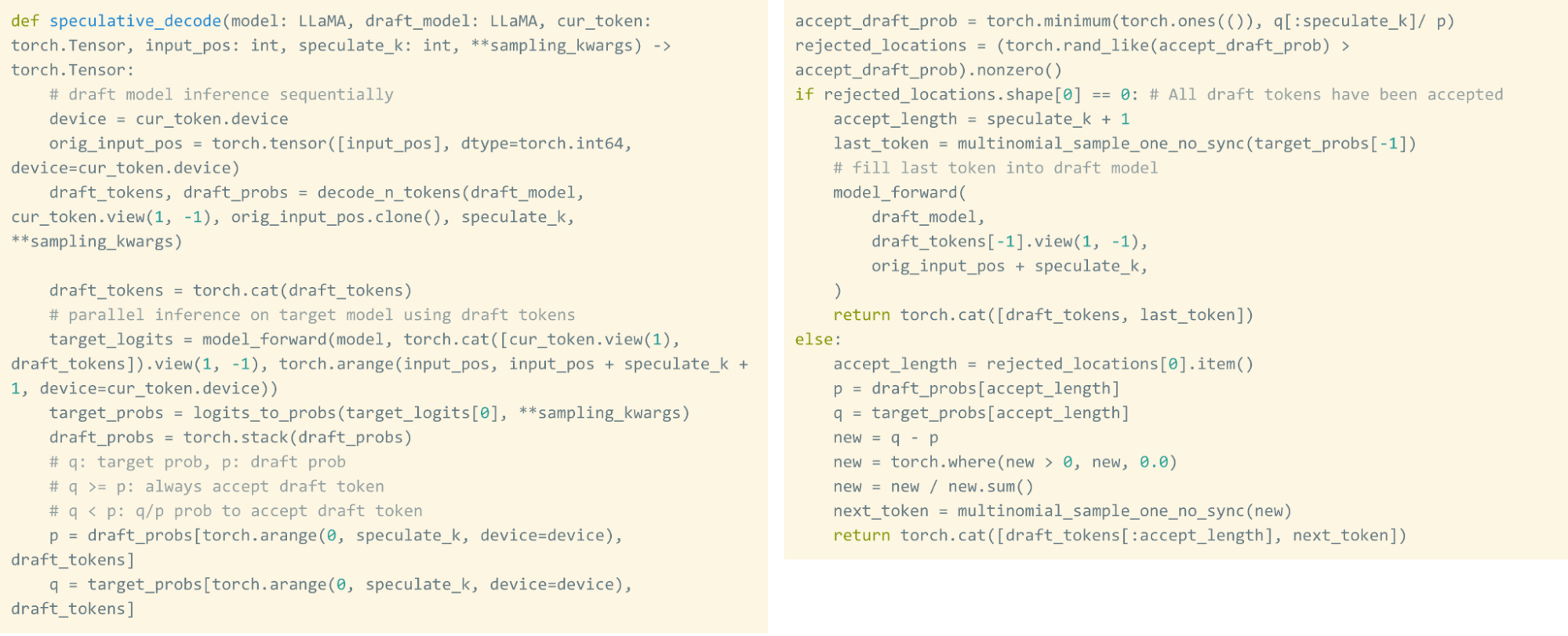
Although speculative decoding guarantees that we have mathematically identical results compared to regular generation, it does have the property that the runtime performance varies depending on the generated text, as well as how aligned the draft and verifier model are. For example, when running CodeLlama-34B + CodeLlama-7B, we’re able to obtain a 2x boost in tokens/s for generating code. On the other hand, when using Llama-7B + TinyLlama-1B, we’re only able to obtain about a 1.3x boost in tokens/s.
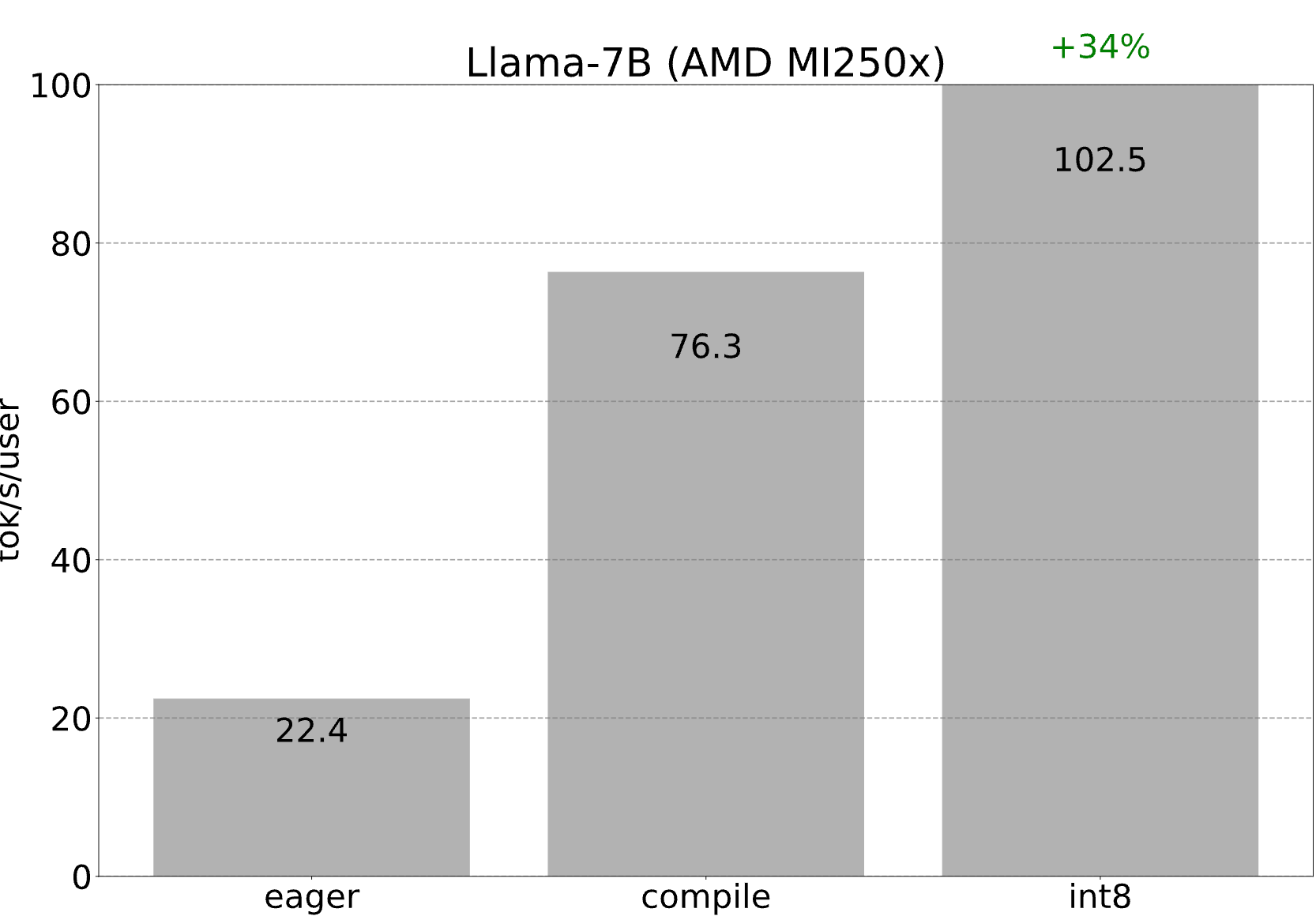
Sidenote: Running this on AMD
Like mentioned above, every single kernel in decoding is generated from scratch by torch.compile, and is converted into OpenAI Triton. As AMD has a torch.compile backend (and also a Triton backend), we can simply go through all of the optimizations above… but on an AMD GPU! With int8 quantization, we’re able to achieve 102.5 tokens/s with one GCD (i.e. one half) of a MI250x!
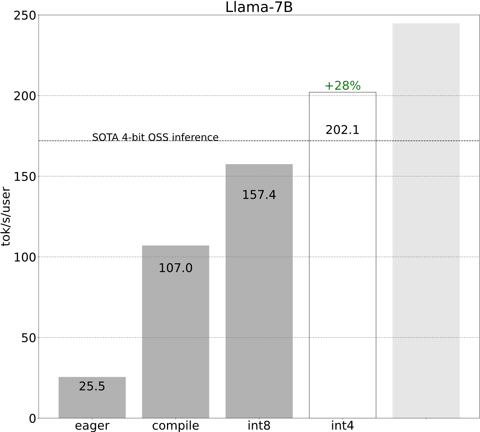
Step 4: Reducing the size of the weights even more with int4 quantization and GPTQ (202.1 tok/s)
Of course, if reducing the weights down from 16 bits to 8 bits allows for speedups by reducing the number of bytes we need to load, reducing the weights down to 4 bits would result in even larger speedups!
Unfortunately, when reducing weights down to 4-bits, the accuracy of the model starts to become a much larger concern. From our preliminary evals, we see that although using int8 weight-only quantization has no perceptible accuracy degradation, using int4 weight-only quantization does.
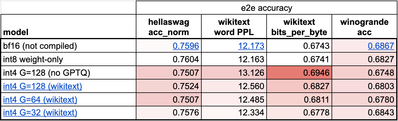
There are 2 main tricks we can use to limit the accuracy degradation of int4 quantization.
The first one is to have a more granular scaling factor. One way to think about the scaling factor is that when we have a quantized tensor representation, it is on a sliding scale between a floating point tensor (each value has a scaling factor) and an integer tensor (no values have a scaling factor). For example, with int8 quantization, we had one scaling factor per row. If we want higher accuracy, however, we can change that to “one scaling factor per 32 elements”. We choose a group size of 32 to minimize accuracy degradation, and this is also a common choice among the community.
The other one is to use a more advanced quantization strategy than simply rounding the weights. For example, approaches like GPTQ leverage example data in order to calibrate the weights more accurately. In this case, we prototype an implementation of GPTQ in the repository based off of PyTorch’s recently released torch.export.
In addition, we need kernels that fuse int4 dequantize with the matrix vector multiplication. In this case, torch.compile is unfortunately not able to generate these kernels from scratch, so we leverage some handwritten CUDA kernels in PyTorch.
These techniques require some additional work, but putting them all together results in even better performance!
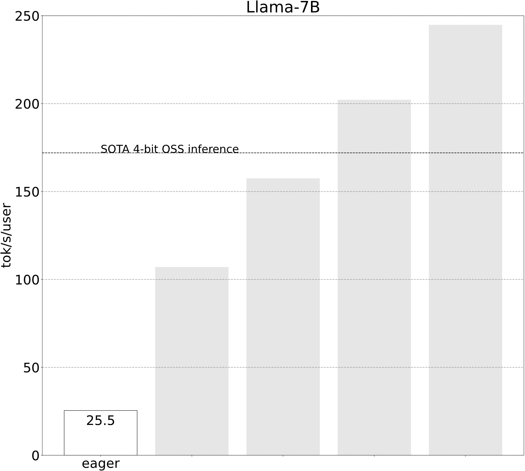
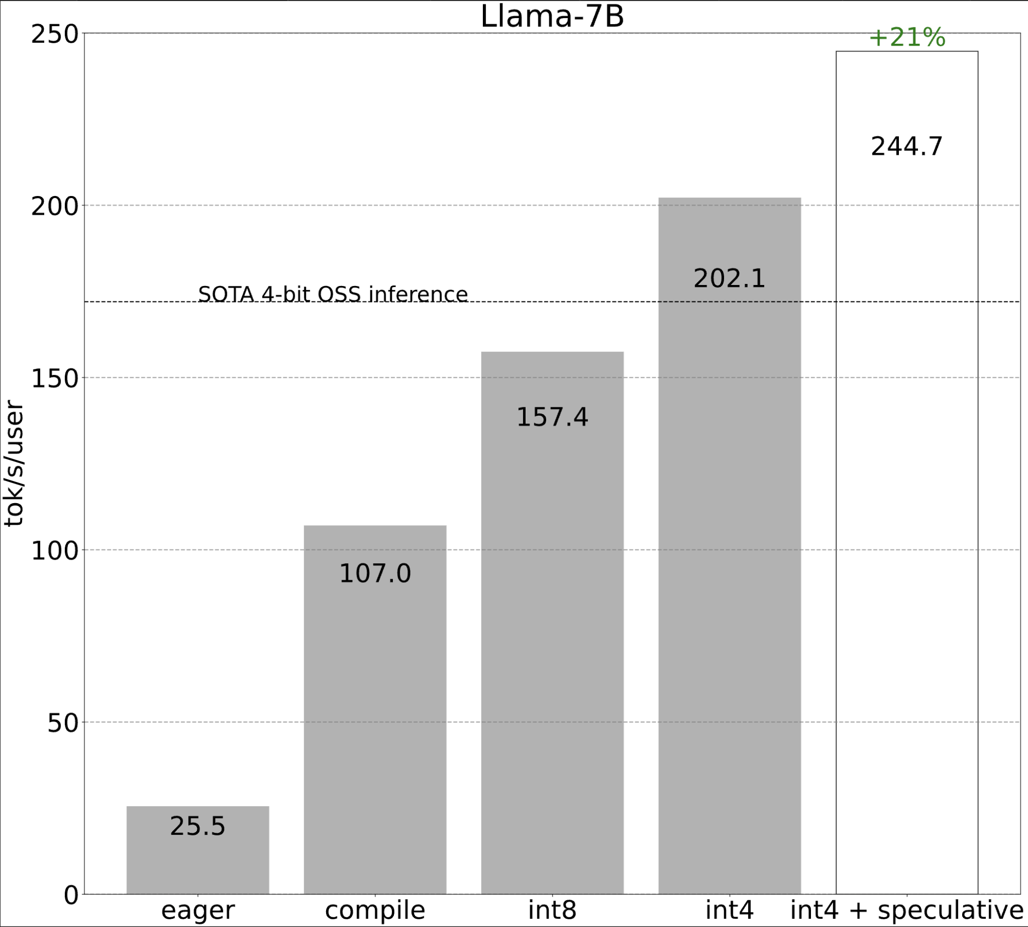
Step 5: Combining everything together (244.7 tok/s)
Finally, we can compose all of the techniques together to achieve even better performance!
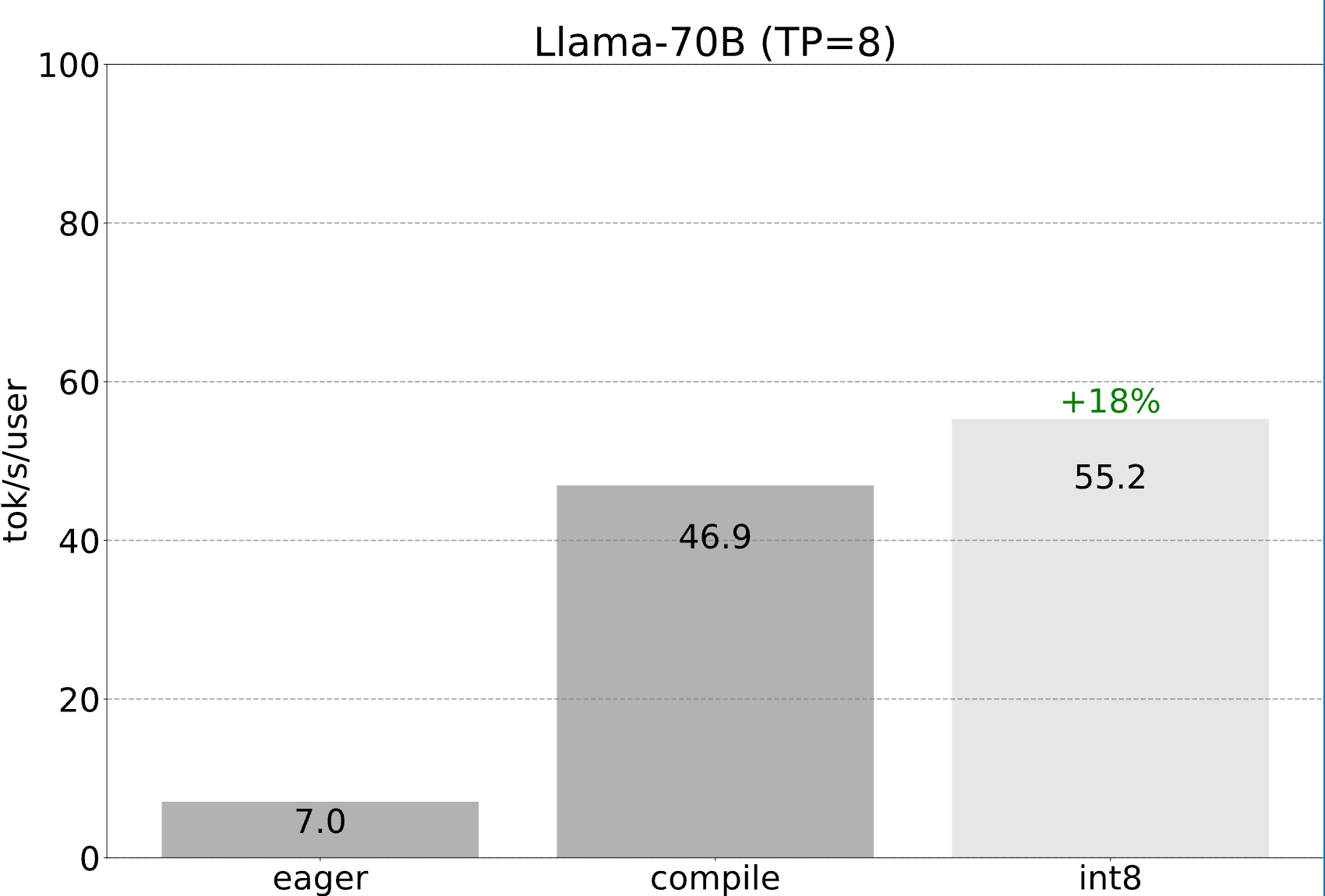
Step 6: Using Tensor Parallelism
So far, we’ve been restricting ourselves to minimizing latency while on a single GPU. In many settings, however, we have access to multiple GPUs. This allows us to improve our latency further!
To get an intuitive sense of why this would allow us to improve our latency, let’s take a look at the prior equation for MBU, particularly the denominator. Running on multiple GPUs gives us access to more memory bandwidth, and thus, higher potential performance.
As for which parallelism strategy to pick, note that in order to reduce our latency for one example, we need to be able to leverage our memory bandwidth across more devices simultaneously. This means that we need to split the processing of one token across multiple devices. In other words, we need to use tensor parallelism.
Luckily, PyTorch also provides low-level tools for tensor-parallelism that compose with torch.compile. We are also working on higher-level APIs for expressing tensor parallelism, stay tuned for those!
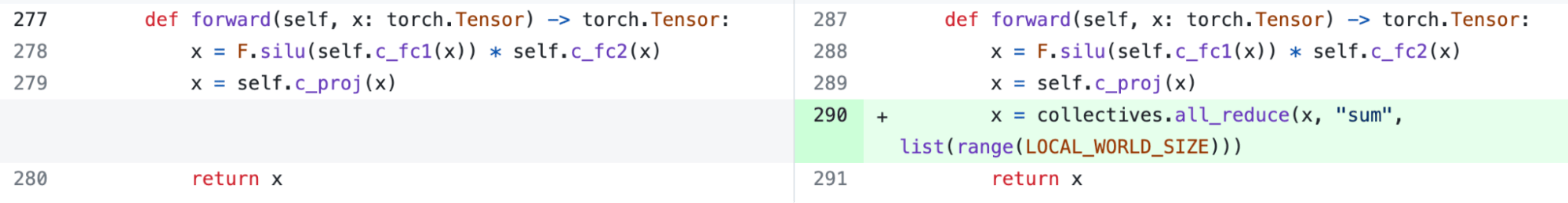
However, even without a higher-level API, it’s actually still quite easy to add tensor parallelism. Our implementation comes in at 150 lines of code, and doesn’t require any model changes.
We are still able to take advantage of all the optimizations mentioned previously, which all can continue to compose with tensor parallelism. Combining these together, we’re able to serve Llama-70B at 55 tokens/s with int8 quantization!
Conclusion
Let’s take a look at what we’re able to accomplish.
- Simplicity: Ignoring quantization, model.py (244 LOC) + generate.py (371 LOC) + tp.py (151 LOC) comes out to 766 LOC to implement fast inference + speculative decoding + tensor-parallelism.
- Performance: With Llama-7B, we’re able to use compile + int4 quant + speculative decoding to reach 241 tok/s. With llama-70B, we’re able to also throw in tensor-parallelism to reach 80 tok/s. These are both close to or surpassing SOTA performance numbers!
PyTorch has always allowed for simplicity, ease of use, and flexibility. However, with torch.compile, we can throw in performance as well.
The code can be found here: https://github.com/pytorch-labs/gpt-fast. We hope that the community finds it useful. Our goal with this repo is not to provide another library or framework for people to import. Instead, we encourage users to copy-paste, fork, and modify the code in the repo.
Acknowledgements
We would like to thank the vibrant open source community for their continual support of scaling LLMs, including:
- Lightning AI for supporting pytorch and work in flash attention, int8 quantization, and LoRA fine-tuning.
- GGML for driving forward fast, on device inference of LLMs
- Andrej Karpathy for spearheading simple, interpretable and fast LLM implementations
- MLC-LLM for pushing 4-bit quantization performance on heterogenous hardware