Featured projects
TL;DR:
- ExecuTorch extends the PyTorch ecosystem to deliver local AI inference on constrained edge devices. To provide a practical entry point, Arm has created a set of Jupyter Labs that complement the official ExecuTorch documentation while explaining both the how and the why of each step.
- The blog and labs introduce both CPU and NPU inference, across Cortex-A and Cortex-M + Ethos-U platforms, and showcase use of Model Explorer adapters, developed by Arm, to gain visibility into model deployment with ExecuTorch.
AI is rapidly and undisputedly becoming part of how we work and live. But today, much of that intelligence is still tied to the cloud, accessed through APIs and web interfaces.
That model doesn’t always fit. Businesses increasingly want to bring AI closer to where it’s actually used—on devices like wearables, smart cameras, and other low-power edge systems. Running AI locally can reduce latency, improve privacy, and unlock new real-time capabilities, but it also introduces a new challenge: how do you run complex models efficiently on constrained hardware with limited memory, compute, and power?
PyTorch has become the foremost framework for training and inferencing AI models in the cloud. ExecuTorch extends that ecosystem to bring local AI inference to the edge. It takes a PyTorch model, exports it into a lightweight format, and runs it through a runtime built specifically for edge inference. If you’re already familiar with PyTorch, the appeal is clear: you stay in the same ecosystem, while gaining a deployment path better suited to real devices.
To make this practical, Arm has created a set of hands-on Jupyter labs that walk through the deployment process—from CPU inference on a Raspberry Pi through to hardware acceleration on Ethos-U NPUs. Whether you’re an ML developer already comfortable with PyTorch or an embedded engineer building your ML foundations, this lab series provides a practical entry point, with executable examples that complement the official ExecuTorch documentation while explaining both the how and the why of each step.
ExecuTorch on Edge CPUs
You may already be familiar with running PyTorch on edge devices like the Raspberry Pi 5. We explore this in our course Optimizing Generative AI on Arm. While this works well, the Pi sits in the category of single-board computers (SBCs), with significantly more resources than many production-grade embedded or IoT systems. For more constrained targets—such as Cortex-M microcontrollers— running PyTorch is not viable due to its size and dependencies.
ExecuTorch addresses this and enables efficient deployment of PyTorch models to edge devices. This is achieved through exporting a model into a minimal .pte artefact containing both the model weights and a static computation graph. This removes the need for Python at runtime and avoids dynamic execution overhead that is unnecessary for inference.
The export step is followed by lowering, where the model graph is transformed into a backend-compatible form. This is where hardware-aware optimization begins.
The resulting artefact is:
- lightweight and portable
- predictable in execution
- suitable for deployment on constrained systems
Beyond the portability of the .pte, there are other benefits. Even on devices like the Raspberry Pi, which can run PyTorch models without needing ExecuTorch, performance improvements can be found through using ExecuTorch. However, performance depends heavily on how the model is executed. ExecuTorch achieves performance by delegating parts of the model to optimized backends.
On Arm CPUs, this is typically done using the XNNPACK backend. When enabled, supported operators—such as convolutions and matrix multiplications—are delegated to highly optimized implementations. On Arm platforms, these implementations leverage KleidiAI microkernels, which make efficient use of architectural features such as Neon. In our labs, we compare inference of an OPT-125M transformer model on a Raspberry Pi 5. The graph below shows a significant latency reduction when using ExecuTorch with XNNPACK:
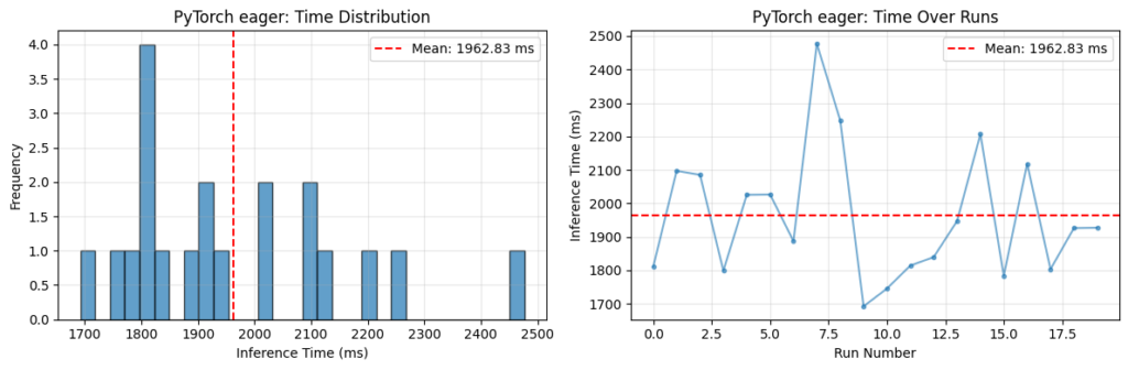
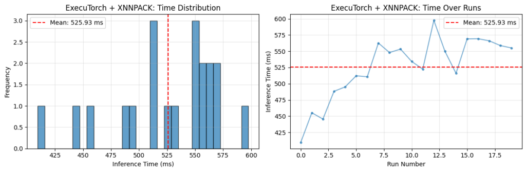
Fig 1. Comparison of PyTorch and ExecuTorch Inference Time on Raspberry Pi 5 CPU
Note: Both PyTorch eager mode and ExecuTorch + XNNPACK were run with several warm-up iterations discarded to avoid the typical pattern of slower initial runs followed by faster steady-state performance.
In the case of ExecuTorch, the opposite trend is observed: the first few measured runs are faster, with latency increasing over subsequent runs. This behaviour is attributed to thermal effects on the Raspberry Pi. Sustained, highly optimized inference with ExecuTorch + XNNPACK places greater load on the CPU, leading to increased temperature and a corresponding reduction in clock speed over time. No active cooling was used during these experiments.
It’s important to note that backend delegation doesn’t occur by default. Running ExecuTorch without XNNPACK will often result in higher latency compared to PyTorch (which has its own KleidiAI optimizations), though you still benefit from a reduced runtime footprint and improved portability.
The key takeaway is that ExecuTorch provides the deployment framework, but backend selection determines how effectively the hardware is utilized.
From CPU to NPU: Ethos-U and TOSA
To go further, we can target hardware acceleration using Arm Ethos-U NPUs, typically paired with Cortex-A or Cortex-M CPUs.
At this point, execution becomes heterogeneous. Rather than running the entire model on one processor, ExecuTorch partitions the graph:
- supported subgraphs are delegated to the NPU
- unsupported operators fall back to the CPU
Ethos-U operates on quantized integer models (typically INT8), so models must be quantized before delegation. The first step is to create a quantizer specific to the backend using EthosUQuantizer and a compile_spec matching your specific target Ethos-U.
For example, the Ethos-U targeted here is an Ethos-U85 with 256 multiply-accumulate (MAC) units:
 compile_spec = EthosUCompileSpec(
target="ethos-u85-256",
system_config="Ethos_U85_SYS_DRAM_Mid",
memory_mode="Shared_Sram",
extra_flags=["--output-format=raw"],
)

quantizer = EthosUQuantizer(compile_spec)
Once a quantizer has been created, the PyTorch 2 Export (PT2E) quantization flow can be performed as normal.
The next step involves lowering the model into TOSA (Tensor Operator Set Architecture), an intermediate representation designed to bridge high-level frameworks and hardware backends. TOSA provides a stable, hardware-agnostic operator set. Instead of requiring each hardware vendor to support every framework-specific operator, models are lowered into TOSA, and hardware backends implement this smaller, standardized set.
This step uses the to_edge_transform_and_lower API, specifying use of the EthosUPartitioner. For Ethos-U this triggers the backend path that serializes to TOSA and runs Vela to produce an optimized command stream for execution on the NPU. Finally, .to_executorch(...) packages the result into a .pte file.
Understanding this flow is useful when analyzing performance. Efficient delegation typically results in large, contiguous subgraphs running on the NPU. If unsupported operators are present, the graph can become fragmented, leading to multiple smaller subgraphs and increased overhead due to frequent transitions between CPU and NPU.
To make this visible, the labs utilize Google’s Model Explorer, along with adapters developed by Arm. These tools allow you to:
- Inspect the ExecuTorch graph (.pte) and visualize how it is partitioned across backends
- Examine the TOSA representation (.tosa)
- You can also visualize VGF (.vgf) files used for the Arm ML SDK for Vulkan® (not covered in the hands-on labs)
For example, below are two .pte files targeting the same Ethos-U configuration, but generated from slightly different models.
The right-hand image shows a MobileNetV2 model with an additional LRN layer inserted. Because LRN is not natively supported, it is decomposed into lower-level operations during lowering. Not all of these operations can be delegated, and the graph is partitioned into multiple segments. Supported regions are delegated to the NPU, while the unsupported portion runs on the CPU. In contrast, the left-hand model is regular MobileNetV2, and contains only supported operators, allowing the entire compute region to be delegated as a single, continuous Ethos-U subgraph.
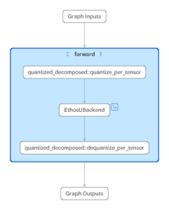
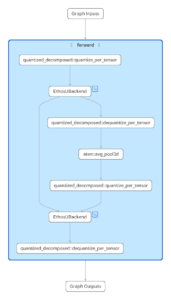
Fig 2. Model Explorer using the PTE Adapter to inspect .pte files targeting Ethos-U for two different models (MobileNetV2, MobileNetV2 + LRN layer)
This level of visibility helps explain performance behavior and can guide optimization decisions.
Practical Next Steps
To get familiar with these topics, we have released a collection of Jupyter labs, designed so you can run and modify the code on your own hardware – making the theory immediately actionable. Take a look here.
This collection includes contributions from Professor Marcelo Rovai (UNIFEI University, and a member of the Edge AI Foundation Academia-Industry Partnership).
Additional thanks go to the academic reviewers at IIIT Bangalore, who ensured the material is rigorously validated and valuable for developers and learners.
For a broader overview of Edge AI Developer Resources provided by Arm, please look here.
Building models is only half the story—getting them running efficiently at the edge is what matters. ExecuTorch makes that possible, and these labs show you how to get started quickly while understanding the underlying concepts.