TL;DR We recently demonstrated a +30.2% training speedup for Llama4 Scout with equivalent convergence to bfloat16, by using MXFP8 MoE training primitives in TorchAO! This is ~81% of the theoretical max achievable speedup for this model training config with the given general matrix multiplications (GEMMs) and grouped GEMMs converted to MXFP8 (roofline 1.37x). These experiments were performed on Crusoe Cloud.
In this blog, we will discuss:
- Training run results and how you can reproduce them with TorchTitan and TorchAO
- An illustrated deep-dive of the forward and backward pass of the dynamically quantized MXFP8 grouped GEMM in MoE training
Convergence experiment and results
Our training runs on a 64 node / 256 device GB200 cluster with TorchTitan Llama4 Scout demonstrated equivalent convergence to the bfloat16 training baseline. This is consistent with our scaling experiments with MXFP8 training for dense models. We used the training configuration below:
- Model: Llama4 Scout
- Dataset: C4
- Sequence length: 8192
- Local batch size: 1
- Learning rate: 1e-4
- LR scheduler warmup steps: 2000
- Parallelisms:
- FSDP=256 (on attention layers, shared experts, dense layer FFNs) and 256/4=64 (on routed experts)
- EP=16 (on routed experts)
- Activation checkpointing mode: full (recompute all intermediate activations instead of storing them, to reduce peak memory requirements)
- torch.compile enabled in TorchTitan on components: model, loss
- mxfp8 applied to routed experts computation (grouped GEMMs)
- mxfp8 applied to all linear layers except those matching the FQNs: output, router.gate, attention.wk, attention.wv
- output embedding projection is too sensitive to low precision, adversely impacts convergence
- Wk/Wv are too small to see a net performance benefit from dynamic mxfp8 quantization
Versions
- torch: 2.11.0.dev20260122+cu130
- torchtitan: 0.2.1
- torchao: 0.17.0+git41e02b5fb
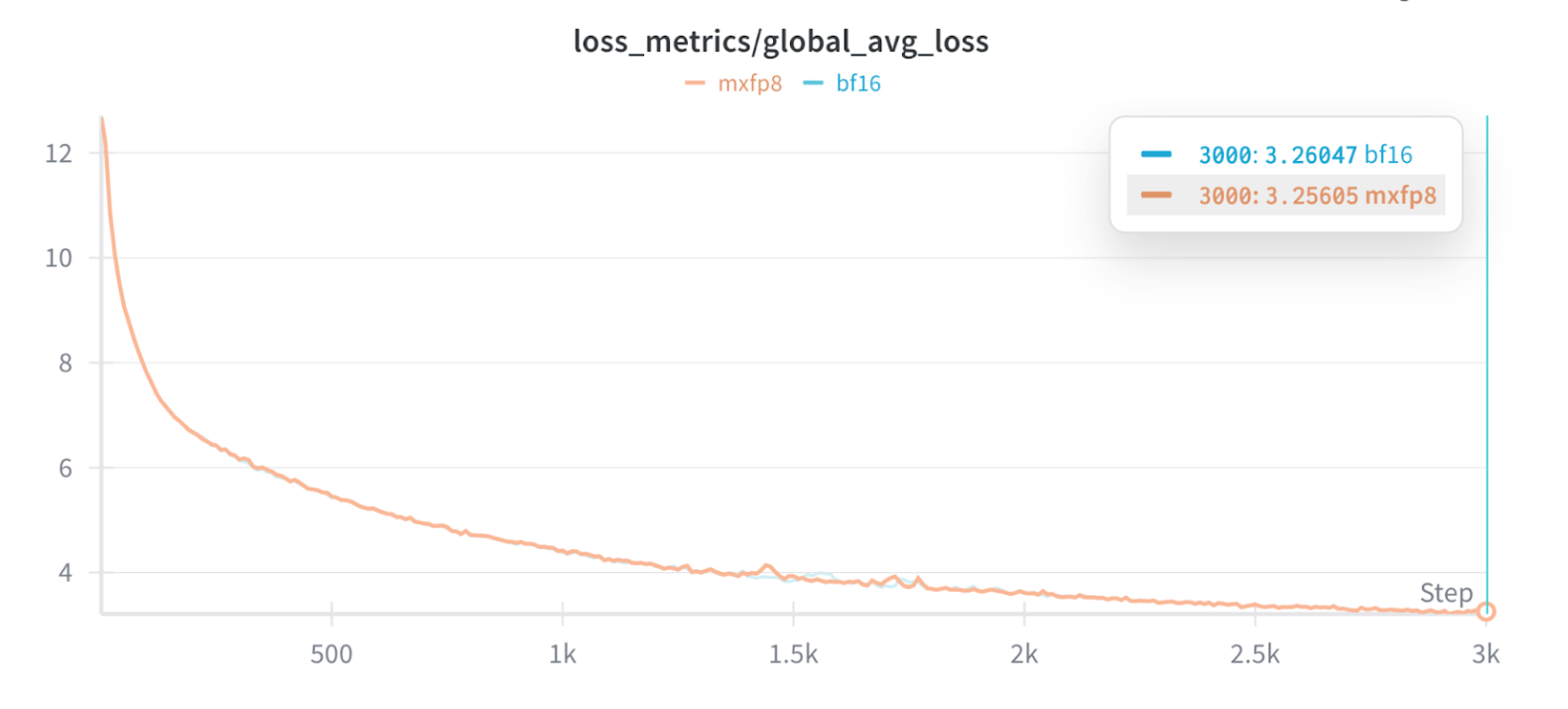
Training loss curves demonstrating equivalent convergence to bf16 for 3k+ steps
We performed a long running convergence experiment (3k steps) to evaluate if the convergence behavior between bfloat16 baseline and mxfp8 is equivalent. In order to keep the time window on the cluster manageable we used a small local batch size of 1 for the run. The depicted loss curves show virtually identical training loss curves.
Performance benchmarks
Next, to evaluate the achievable performance improvements with MXFP8, we increased the local batch size from 1 to 16, as is typical for improving GEMM efficiency in sparsely activated MoEs. This resulted in an end-to-end training speedup of +30.2% over bf16 with equivalent configs.
| Number of GPUs | BF16 tokens/sec | MXFP8 tokens/sec | MXFP8 speedup vs BF16 |
| 256 | 5317 | 6921 | 30.2% |
The engine powering this speedup is the _to_mxfp8_then_scaled_grouped_mm op that is ~1.8x faster than compiled bf16 for these shapes. Using this for routed experts results in a 1.43x faster MOE layer and 1.2x faster e2e training with Llama4 Scout vs compiled bf16. Additionally, when we use MXFP8 for the shared expert linear layers as well, we reach 1.3x e2e training speedup vs compiled bf16. See the Appendix for microbenchmark tables.
In the next section we will give an introduction of the TorchAO APIs as well as give further technical details on mxfp8 and its application in scaled grouped GEMMs.
TorchTitan Config for MXFP8 MoE training
For the results of the previous section we relied on TorchTitan as our training framework. To use MXFP8 training for MoEs in TorchTitan, check out the documentation which details the necessary configs and examples.
TorchAO MXFP8 MoE training APIs
If you’re not using TorchTitan, you can also use the TorchAO primitives directly. TorchAO recently added a prototype API, _to_mxfp8_then_scaled_grouped_mm, which does exactly what it sounds like: quantizes grouped GEMM inputs (activations and weights) to mxfp8, then does a scaled grouped GEMM with the mxfp8 operands, producing an output in the original precision. This primitive is differentiable so can be used for training out of the box. Check out the docs for detailed microbenchmarks, roofline analysis for shapes used in different popular models, and more.
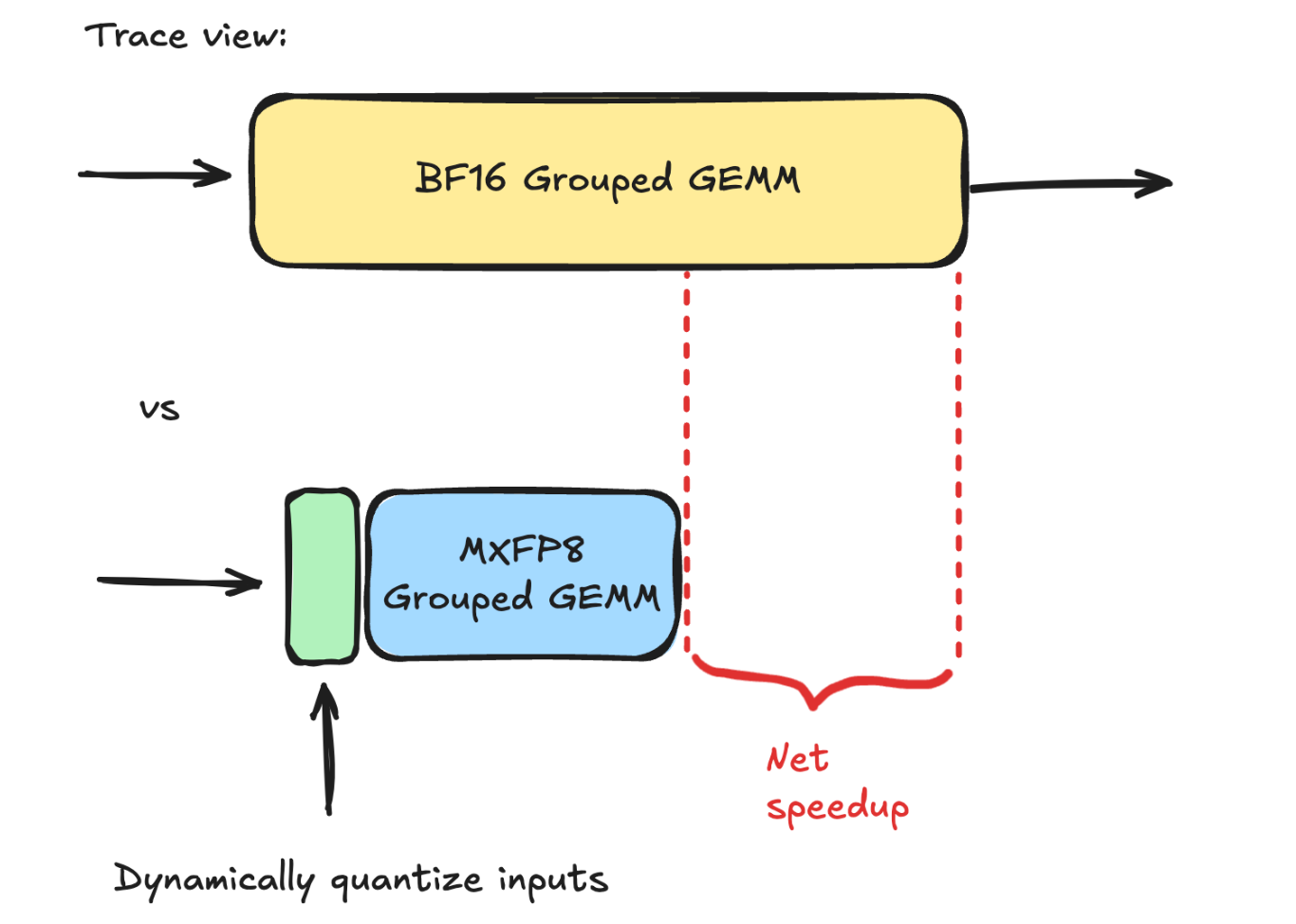
The goal of this primitive is to achieve a net speedup over the bf16 grouped GEMM baseline. By dynamically quantizing the inputs to mxfp8, we can then use a mxfp8 scaled grouped GEMM, which achieves up to 2x higher TFLOPs/sec vs bf16. Thus, as long as our quantization kernels are sufficiently fast and don’t introduce excessive overhead, we should be able to achieve a net speedup, as shown in the diagram below:
Illustrated walkthrough of a forward and backward pass through dynamic MXFP8 quantization + scaled grouped GEMM
Let’s do a tour through the forward and backward pass, starting at the moment our input activations come in to go through the forward pass of the routed experts!
Our starting point is immediately before the routed expert computation in the MoE layer. To be clear, at this point in the execution of the MoE layer, the following steps have already happened:
- The expert affinity scores for each token have been computed by the router (token choice routing)
- Tokens have been “assigned” to top K experts based on the scores
- For expert parallelism, all-to-all comms dispatch tokens to the device the target expert resides on
- Each device does a token shuffle/permutation such that tokens are grouped by expert and the groups are sorted in the same order as the expert weights
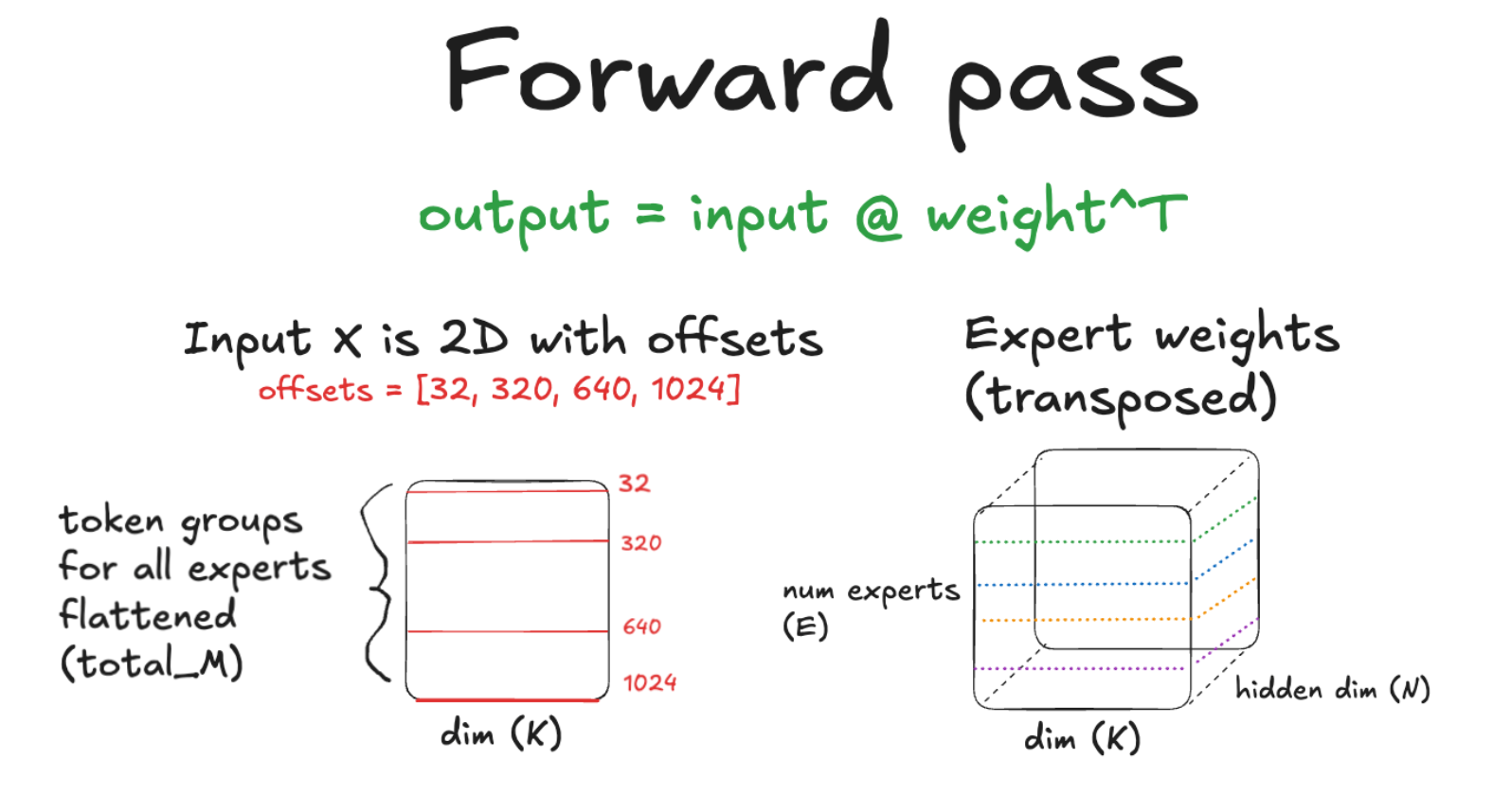
- This shuffle operation produces a tensor called the offsets tensor, which stores the end index of each group in the flattened 2d tensor of token group
So we have our high precision input activations and weights for the routed experts as shown below.
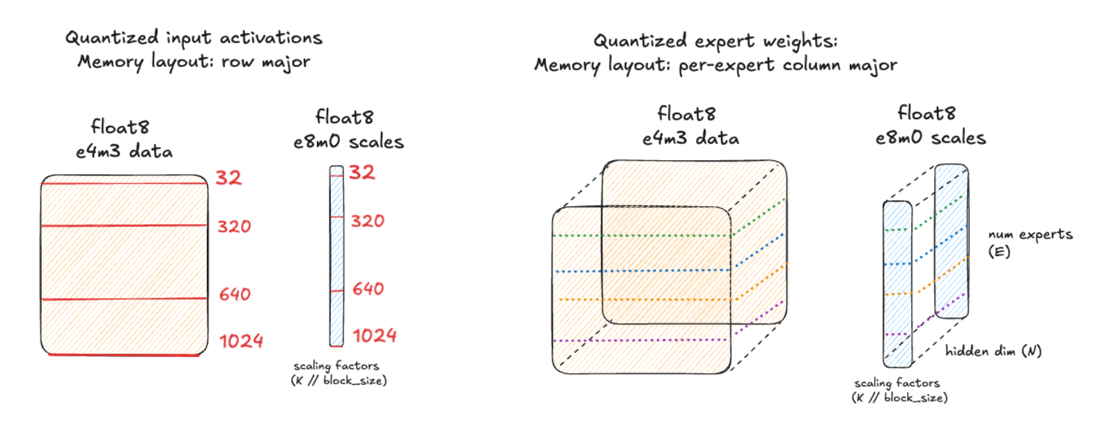
MXFP8 quantization
This is the key point where we will now dynamically quantize the input activations and weights to MXFP8, giving us float8 e4m3 data and float8 e8m0 scale factor.
Each 1×32 chunk of high precision input data shares a single e8m0 scale factor value that is used to scale the values to fill the dynamic range of the float8 e4m3 data type.
Write per-group scale factors to blocked layout with group boundaries along rows (M)
To do efficient grouped GEMMs on Blackwell GPUs, we’ll want our kernel to use the hardware’s 5th generation tensorcores, which are key to maximizing the compute throughput (TFLOPs/sec) on these chips. These tensorcores are programmed using the tcgen05 family of PTX instructions, which are the assembly-like instructions that familiar kernel languages like CUDA will be lowered to as part of the compilation.
For MXFP8 grouped GEMMs specifically, we’ll need to use the block scaled variant of the tcgen05.mma PTX instructions. This instruction has some peculiar requirements for the layout of the e8m0 scale factors in our MXFP8 data.
Specifically, the scale factors must reside in tensor memory (TMEM) in an unconventional blocked layout, which can be seen in the NVIDIA docs here:
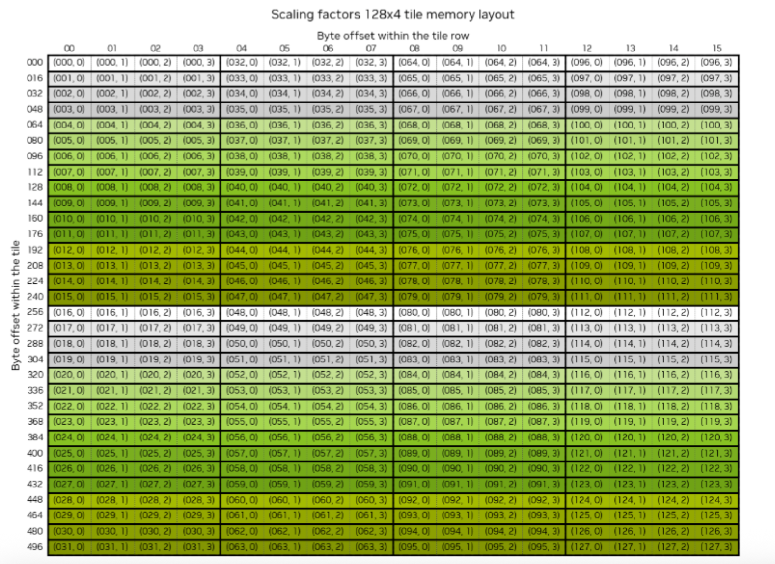
Source: https://docs.nvidia.com/cuda/cublas/index.html#d-block-scaling-factors-layout
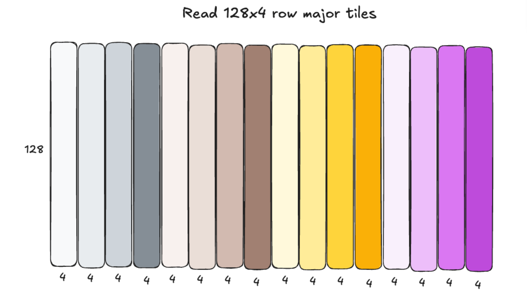
Therefore, in our quantization kernels, we need write the scale factors to this layout so they are usable by the tenscores. To convert the scales from simple row-major layout to this blocked layout, we want to do 3 things:
- Pad each token group’s scales such that they are evenly divisible into 128×4 tiles.
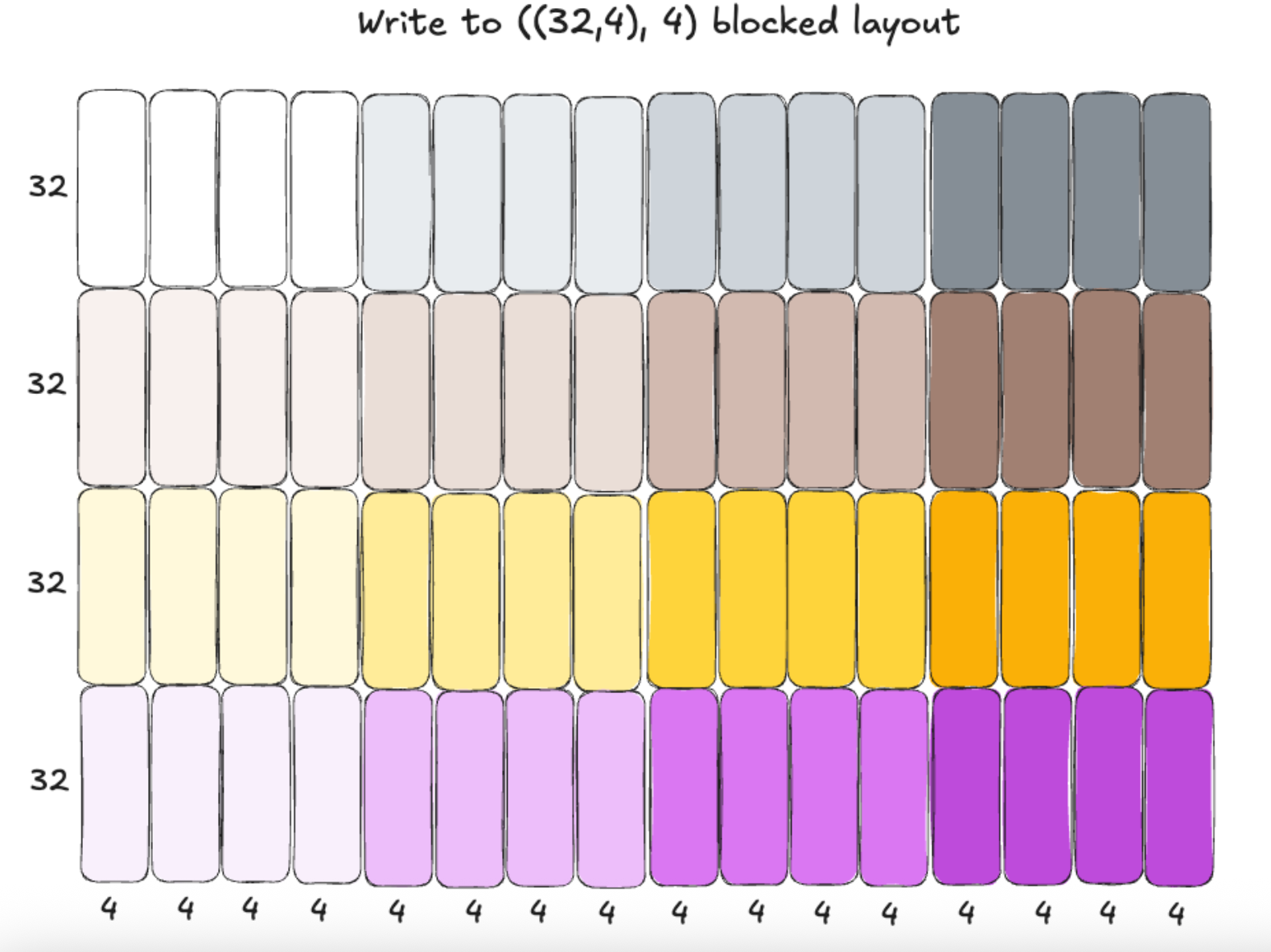
- Within each 128×4 tile, apply a layout transformation from simple row major to a ((32,4), 4) layout, meaning we have 4 (32,4) tiles logically arranged horizontally to each other in memory. You can think of it as a (32,16) shaped tensor where each 16 byte “super row” now contains 4 rows, one from each tile. These superrows are contiguous in memory.
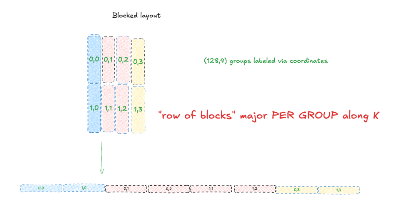
- Writes out these tiles with tile-level granularity to a “row of blocks” major layout, as shown below (e.g., we write out the full tile as contiguous memory before proceeding to the next tile along the row)
Here is a before/after diagram of this blocked layout transformation that visualizes it a bit better. For more details, you can refer to the NVIDIA documentation.
When accounting for groups, the actual memory layout looks like this. Groups are along the M dimension (rows) for the 2d-3d MXFP8 grouped GEMM in the forward pass:
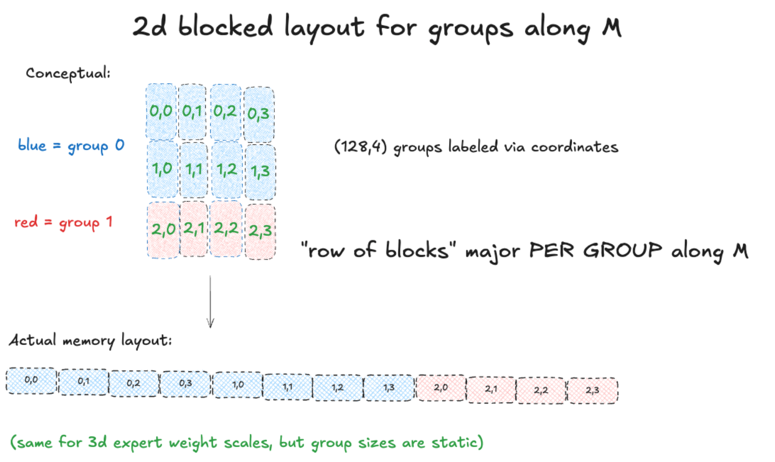
Transformation to this unconventional layout will need to be done very carefully to avoid incurring excessive overhead that will kill our net speedup (or worse, cause a slowdown!).
But wait – there’s more! This is only accounting for a single scale factor. Remember, we are doing a grouped GEMM which parallelizes our routed expert GEMMs and executes them in a single kernel. The data and scales for each GEMM live in the same tensor, but all must be individually valid for the tcgen05.mma PTX instruction we talked about. This means that we cannot directly apply the layout transformation on the scale tensor directly; rather, we need to do this layout conversion on each individual group separately.
Furthermore, the token group sizes for each expert are dynamic, and known only on the device! This means from our host side PyTorch code we can dispatch kernels to transform each group’s memory layout separately, because the host does not have group size information. To get it would require a host device sync, causing a large gap (idle time) in our GPU kernel execution stream, which would be terrible for performance! Therefore, we must design a custom kernel that can perform this task purely on the device side efficiently.
It turns out this is a very interesting and unusual kernel to write – one that warrants a separate deep dive post. In the meantime, let’s move onto the next step of our MXFP8 Grouped GEMM after we’ve dynamically quantized our inputs and written the scale factors to per group blocked layout.
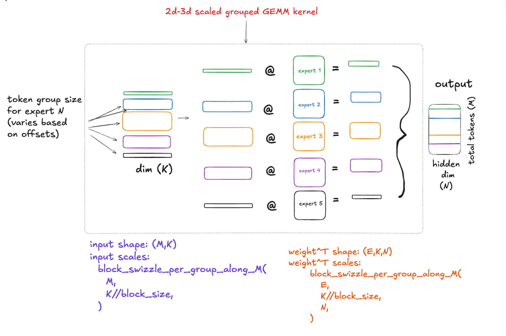
2d–3d MXFP8 Grouped GEMM for forward output
With our data and scales in place in the proper memory layouts, we are finally ready to do our MXFP8 Grouped GEMM between our 2d input activations and 3d weights! This gives us a 2d output where each token has been projected to the hidden dimension. Decomposed, it looks like this:
 Backward pass; 2d–3d MXFP8 Grouped GEMM for input gradient computation
The gradient of the input is fairly similar to the 2D 3D scaled group GEMM for the forward output, so we won’t go into much detail here as this is already getting quite lengthy. Specifically, the formula is:
dgrad = dO @ weight
The gradient of our output has the same shape as our forward output. So it is a 2D tensor of shape (total_M, N). Our weight is still our weight, a 3D tensor of shape (E,N,K).
So we quantize our 2D output gradient the same way we quantized our input activations in the forward pass, and we quantize our weights very similarly. Except this time they are non-transposed, in row-major format, and we are writing them to per-expert column-major format. So the kernel is a bit different, but that’s the only difference.
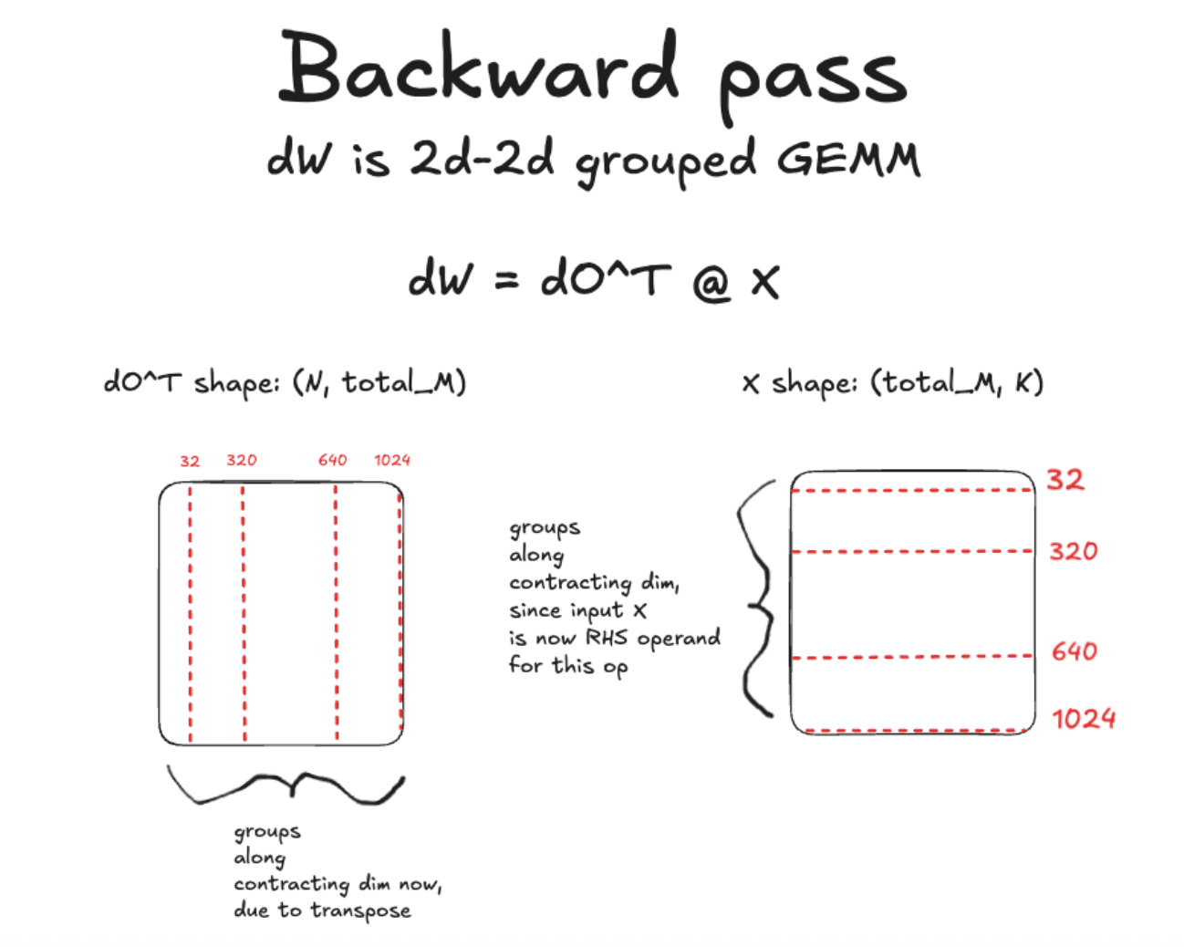
Backward pass; 2d–2d MXFP8 Grouped GEMM for weight gradient computation
The gradient of the weight is more interesting to discuss. This is because it involves an entirely different type of grouped GEMM, with different challenges. The formula for calculating the gradient of the weights is:
dW = dO^T @ X
This is a 2d-2d grouped GEMM with shapes (N, total_M) @ (total_M,K). As you can see, the groups are now along the contracting dimension of the GEMMs!
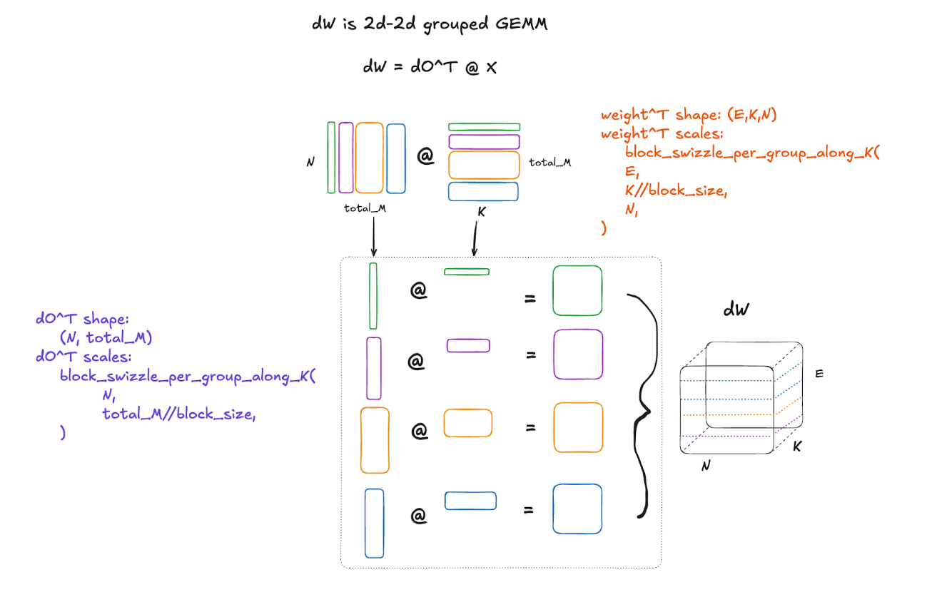
Writing per group scale factors to blocked format with groups along the contracting dimension (K)
How does this change things? Well, a kernel that converts scales to block format with groups along the m dimension, or the rows, is now no longer quite right for this case, where the groups are along the contracting or K dimension. This is because the input scale is in a row-major layout, and so slicing the tensor up into groups along column boundaries fundamentally changes the strides and makes the strides dynamic per group. So we need a kernel that handles the case of different strides per group. In this case, we need to calculate the number of 128×4 tiles along each row in the group, and our stride will be the stride per tile times the number of tiles along a row in that group. It sounds complicated, and it is, but here is a diagram to help visualize and make this a bit simpler to understand:
Each individual GEMM in the grouped GEMM produces a 2d output which are stacked into the final 3d result. Decomposed, it looks like this:
And there we have it! At this point, hopefully you have a better understanding of what’s going on under the hood in both the forward and backward pass of a dynamically quantized MXFP8 Grouped GEMM!
That’s all for now – we hope you enjoyed the read, and remember to check out the TorchAO MoE training docs which have benchmarks, examples, and more to get started with!
Future work
MXFP8 MoE training in TorchAO is still a prototype feature, and we are actively working on a few improvements before graduating it to stable, namely:
- Unify APIs for MXFP8 training for dense and sparse/MoE models: today, TorchAO has separate APIs for converting a model’s nn.Linear layers and torch._grouped_mm ops to use MXFP8. We are working on unifying these APIs to simplify the UX.
- MXFP8 for expert parallel comms: Furthermore, beyond just the MXFP8 grouped GEMM, we have prototypes of autograd functions for efficient training with expert parallelism that quantize to MXFP8 earlier, before the all-to-all comms and stay in MXFP8 through the grouped GEMMs, thus saving network bandwidth and producing a speedup. Stay tuned for a post on this soon!
Appendix
Microbenchmarks: net speedup of dynamic MXFP8 quantization + MXFP8 grouped GEMM versus bf16 grouped GEMM
Below are some microbenchmarks comparing the combined duration of the forward and backward pass of the autograd function powering MXFP8 MoE training, versus the bf16 torch._grouped_mm baseline, for shapes used in recent MoE model architectures.
M = local_batch_size * sequence_length
G = number_of_experts_on_local_rank
N, K = expert_dimensions
Llama4 Scout shapes
| M,N,K,G | BF16 forward + backward (microseconds) | MXFP8 forward + backward (microseconds) | MXFP8 speedup vs BF16 |
| (128000, 8192, 5120, 1) | 43140.20 | 23867.00 | 1.808x |
| (128000, 8192, 5120, 2) | 39487.60 | 23359.00 | 1.690x |
| (128000, 8192, 5120, 4) | 39189.20 | 23945.50 | 1.637x |
| (128000, 8192, 5120, 8) | 37700.70 | 22170.60 | 1.700x |
You can refer to the documentation for commands to reproduce these benchmarks on a B200 GPU.
MoE layer benchmarks
Microbenchmarks of a single MoE layer on a single B200 also show MXFP8 achieves up to 1.43x faster MoE layer execution vs the bf16 baseline.
| Model | total_M | N | K | bf16 time (ms) | mxfp8 time (ms) | speedup |
| Llama4 16e | 131072 | 8192 | 5120 | 275.270 | 192.420 | 1.431x |
You can refer to the documentation for commands to reproduce these benchmarks on a B200 GPU.