PathAI is the leading provider of AI-powered technology tools and services for pathology (the study of disease). Our platform was built to enable substantial improvements to the accuracy of diagnosis and the measurement of therapeutic efficacy for complex diseases, leveraging modern approaches in machine learning like image segmentation, graph neural networks, and multiple instance learning.

Traditional manual pathology is prone to subjectivity and observer variability that can negatively affect diagnoses and drug development trials. Before we dive into how we use PyTorch to improve our diagnosis workflow, let us first lay out the traditional analog Pathology workflow without machine learning.
How Traditional Biopharma Works
There are many avenues that biopharma companies take to discover novel therapeutics or diagnostics. One of those avenues relies heavily on the analysis of pathology slides to answer a variety of questions: how does a particular cellular communication pathway work? Can a specific disease state be linked to the presence or lack of a particular protein? Why did a particular drug in a clinical trial work for some patients but not others? Might there be an association between patient outcomes and a novel biomarker?
To help answer these questions, biopharma companies rely on expert pathologists to analyze slides and help evaluate the questions they might have.
As you might imagine, it takes an expert board certified pathologist to make accurate interpretations and diagnosis. In one study, a single biopsy result was given to 36 different pathologists and the outcome was 18 different diagnoses varying in severity from no treatment to aggressive treatment necessary. Pathologists also often solicit feedback from colleagues in difficult edge cases. Given the complexity of the problem, even with expert training and collaboration, pathologists can still have a hard time making a correct diagnosis. This potential variance can be the difference between a drug being approved and it failing the clinical trial.
How PathAI utilizes machine learning to power drug development
PathAI develops machine learning models which provide insights for drug development R&D, for powering clinical trials, and for making diagnoses. To this end, PathAI leverages PyTorch for slide level inference using a variety of methods including graph neural networks (GNN) as well as multiple instance learning. In this context, “slides” refers to full size scanned images of glass slides, which are pieces of glass with a thin slice of tissue between them, stained to show various cell formations. PyTorch enables our teams using these different methodologies to share a common framework which is robust enough to work in all the conditions we need. PyTorch’s high level, imperative, and pythonic syntax allows us to prototype models quickly and then take those models to scale once we have the results we want.
Multi-instance learning on gigabyte images
One of the uniquely challenging aspects of applying ML to pathology is the immense size of the images. These digital slides can often be 100,000 x 100,000 pixels or more in resolution and gigabytes in size. Loading the full image in GPU memory and applying traditional computer vision algorithms on them is an almost impossible task. It also takes both a considerable amount of time and resources to have a full slide image (100k x 100k) annotated, especially when annotators need to be domain experts (board-certified pathologists). We often build models to predict image-level labels, like the presence of cancer, on a patient slide which covers a few thousand pixels in the whole image. The cancerous area is sometimes a tiny fraction of the entire slide, which makes the ML problem similar to finding a needle in a haystack. On the other hand, some problems like the prediction of certain histological biomarkers require an aggregation of information from the whole slide which is again hard due to the size of the images. All these factors add significant algorithmic, computational, and logistical complexity when applying ML techniques to pathology problems.
Breaking down the image into smaller patches, learning patch representations, and then pooling those representations to predict an image-level label is one way to solve this problem as is depicted in the image below. One popular method for doing this is called Multiple Instance Learning (MIL). Each patch is considered an ‘instance’ and a set of patches forms a ‘bag’. The individual patch representations are pooled together to predict a final bag-level label. Algorithmically, the individual patch instances in the bag do not require labels and hence allow us to learn bag-level labels in a weakly-supervised way. They also use permutation invariant pooling functions which make the prediction independent of the order of patches and allows for an efficient aggregation of information. Typically, attention based pooling functions are used which not only allow for efficient aggregation but also provide attention values for each patch in the bag. These values indicate the importance of the corresponding patch in the prediction and can be visualized to better understand the model predictions. This element of interpretability can be very important to drive adoption of these models in the real world and we use variations like Additive MIL models to enable such spatial explainability. Computationally, MIL models circumvent the problem of applying neural networks to large image sizes since patch representations are obtained independently of the size of the image.
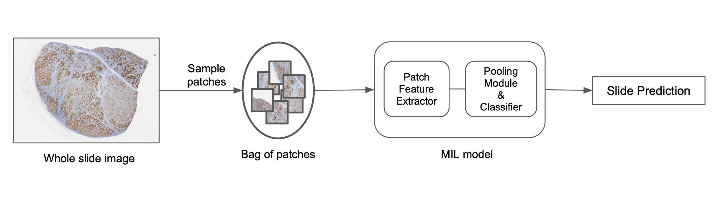
At PathAI, we use custom MIL models based on deep nets to predict image-level labels. The overview of this process is as follows:
- Select patches from a slide using different sampling approaches.
- Construct a bag of patches based on random sampling or heuristic rules.
- Generate patch representations for each instance based on pre-trained models or large-scale representation learning models.
- Apply permutation invariant pooling functions to get the final slide-level score.
Now that we have walked through some of the high-level details around MIL in PyTorch, let’s look at some code to see how simple it is to go from ideation to code in production with PyTorch. We begin by defining a sampler, transformations, and our MIL dataset:
# Create a bag sampler which randomly samples patches from a slide
bag_sampler = RandomBagSampler(bag_size=12)

# Setup the transformations
crop_transform = FlipRotateCenterCrop(use_flips=True)

# Create the dataset which loads patches for each bag
train_dataset = MILDataset(
  bag_sampler=bag_sampler,
  samples_loader=sample_loader,
  transform=crop_transform,
)
After we have defined our sampler and dataset, we need to define the model we will actually train with said dataset. PyTorch’s familiar model definition syntax makes this easy to do while also allowing us to create bespoke models at the same time.
classifier = DefaultPooledClassifier(hidden_dims=[256, 256], input_dims=1024, output_dims=1)

pooling = DefaultAttentionModule(
  input_dims=1024,
  hidden_dims=[256, 256],
  output_activation=StableSoftmax()
)

# Define the model which is a composition of the featurizer, pooling module and a classifier
model = DefaultMILGraph(featurizer=ShuffleNetV2(), classifier=classifier, pooling = pooling)
Since these models are trained end-to-end, they offer a powerful way to go directly from a gigapixel whole slide image to a single label. Due to their wide applicability to different biological problems, two aspects of their implementation and deployment are important:
- Configurable control over each part of the pipeline including the data loaders, the modular parts of the model, and their interaction with each other.
- Ability to rapidly iterate through the ideate-implement-experiment-productionize loop.
PyTorch has various advantages when it comes to MIL modeling. It offers an intuitive way to create dynamic computational graphs with flexible control flow which is great for rapid research experimentation. The map-style datasets, configurable sampler and batch-samplers allow us to customize how we construct bags of patches, enabling faster experimentation. Since MIL models are IO heavy, data parallelism and pythonic data loaders make the task very efficient and user friendly. Lastly, the object-oriented nature of PyTorch enables building of reusable modules which aid in the rapid experimentation, maintainable implementation and ease of building compositional components of the pipeline.
Exploring spatial tissue organization with GNNs in PyTorch
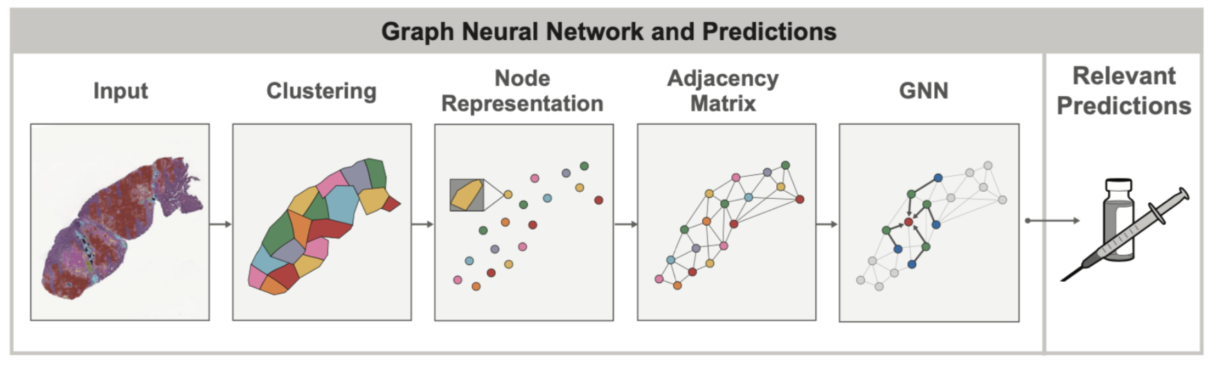
In both healthy and diseased tissue, the spatial arrangement and structure of cells can oftentimes be as important as the cells themselves. For example, when assessing lung cancers, pathologists try to look at the overall grouping and structure of tumor cells (do they form solid sheets? Or do they occur in smaller, localized clusters?) to determine if the cancer belongs to specific subtypes which can have vastly different prognosis. Such spatial relationships between cells and other tissue structures can be modeled using graphs to capture tissue topology and cellular composition at the same time. Graph Neural Networks (GNNs) allow learning spatial patterns within these graphs that relate to other clinical variables, for example overexpression of genes in certain cancers.
In late 2020, when PathAI started using GNNs on tissue samples, PyTorch had the best and most mature support for GNN functionality via the PyG package. This made PyTorch the natural choice for our team given that GNN models were something that we knew would be an important ML concept we wanted to explore.
One of the main value-adds of GNN’s in the context of tissue samples is that the graph itself can uncover spatial relationships that would otherwise be very difficult to find by visual inspection alone. In our recent AACR publication, we showed that by using GNNs, we can better understand the way the presence of immune cell aggregates (specifically tertiary lymphoid structures, or TLS) in the tumor microenvironment can influence patient prognosis. In this case, the GNN approach was used to predict expression of genes associated with the presence of TLS, and identify histological features beyond the TLS region itself that are relevant to TLS. Such insights into gene expression are difficult to identify from tissue sample images when unassisted by ML models.
One of the most promising GNN variations we have had success with is self attention graph pooling. Let’s take a look at how we define our Self Attention Graph Pooling (SAGPool) model using PyTorch and PyG:
class SAGPool(torch.nn.Module):
  def __init__(self, ...):
    super().__init__()
    self.conv1 = GraphConv(in_features, hidden_features, aggr='mean')
    self.convs = torch.nn.ModuleList()
    self.pools = torch.nn.ModuleList()
    self.convs.extend([GraphConv(hidden_features, hidden_features, aggr='mean') for i in range(num_layers - 1)])
    self.pools.extend([SAGPooling(hidden_features, ratio, GNN=GraphConv, min_score=min_score) for i in range((num_layers) // 2)])
    self.jump = JumpingKnowledge(mode='cat')
    self.lin1 = Linear(num_layers * hidden_features, hidden_features)
    self.lin2 = Linear(hidden_features, out_features)
    self.out_activation = out_activation
    self.dropout = dropout
In the above code, we begin by defining a single convolutional graph layer and then add two module list layers which allow us to pass in a variable number of layers. We then take our empty module list and append a variable number of GraphConv layers followed by a variable number of SAGPooling layers. We finish up our SAGPool definition by adding a JumpingKnowledge Layer, two linear layers, our activation function, and our dropout value. PyTorch’s intuitive syntax allows us to abstract away the complexity of working with state of the art methods like SAG Poolings while also maintaining the common approach to model development we are familiar with.
Models like our SAG Pool one described above are just one example of how GNNs with PyTorch are allowing us to explore new and novel ideas. We also recently explored multimodal CNN – GNN hybrid models which ended up being 20% more accurate than traditional Pathologist consensus scores. These innovations and interplay between traditional CNNs and GNNs are again enabled by the short research to production model development loop.
Improving Patient Outcomes
In order to achieve our mission of improving patient outcomes with AI-powered pathology, PathAI needs to rely on an ML development framework that (1) facilitates quick iteration and easy extension (i.e. Model configuration as code) during initial phases of development and exploration (2) scales model training and inference to massive images (3) easily and robustly serves models for production uses of our products (in clinical trials and beyond). As we’ve demonstrated, PyTorch offers us all of these capabilities and more. We are incredibly excited about the future of PyTorch and cannot wait to see what other impactful challenges we can solve using the framework.