Oscillator and ADSR envelope

Author: Moto Hira

This tutorial shows how to synthesize various waveforms using oscillator_bank() and adsr_envelope().

Warning

This tutorial requires prototype DSP features, which are available in nightly builds.

Please refer to https://pytorch.org/get-started/locally for instructions for installing a nightly build.

import torch
import torchaudio

print(torch.__version__)
print(torchaudio.__version__)

2.4.0
2.4.0

try:
    from torchaudio.prototype.functional import adsr_envelope, oscillator_bank
except ModuleNotFoundError:
    print(
        "Failed to import prototype DSP features. "
        "Please install torchaudio nightly builds. "
        "Please refer to https://pytorch.org/get-started/locally "
        "for instructions to install a nightly build."
    )
    raise

import math

import matplotlib.pyplot as plt
from IPython.display import Audio

PI = torch.pi
PI2 = 2 * torch.pi

Oscillator Bank

Sinusoidal oscillator generates sinusoidal waveforms from given amplitudes and frequencies.

\[x_t = A_t \sin \theta_t\]

Where the phase \(\theta_t\) is found by integrating the instantaneous frequency \(f_t\).

\[\theta_t = \sum_{k=1}^{t} f_k\]

Note

Why integrate the frequencies? Instantaneous frequency represents the velocity of oscillation at given time. So integrating the instantaneous frequency gives the displacement of the phase of the oscillation, since the start. In discrete-time signal processing, integration becomes accumulation. In PyTorch, accumulation can be computed using torch.cumsum().

torchaudio.prototype.functional.oscillator_bank() generates a bank of sinsuoidal waveforms from amplitude envelopes and instantaneous frequencies.

Simple Sine Wave

Let’s start with simple case.

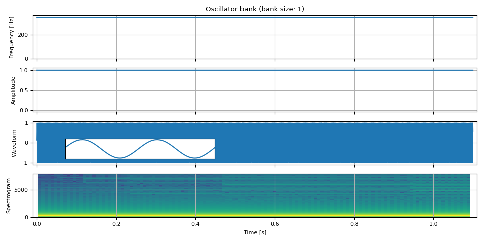
First, we generate sinusoidal wave that has constant frequency and amplitude everywhere, that is, a regular sine wave.

We define some constants and helper function that we use for the rest of the tutorial.

F0 = 344.0  # fundamental frequency
DURATION = 1.1  # [seconds]
SAMPLE_RATE = 16_000  # [Hz]

NUM_FRAMES = int(DURATION * SAMPLE_RATE)

def show(freq, amp, waveform, sample_rate, zoom=None, vol=0.3):
    t = (torch.arange(waveform.size(0)) / sample_rate).numpy()

    fig, axes = plt.subplots(4, 1, sharex=True)
    axes[0].plot(t, freq.numpy())
    axes[0].set(title=f"Oscillator bank (bank size: {amp.size(-1)})", ylabel="Frequency [Hz]", ylim=[-0.03, None])
    axes[1].plot(t, amp.numpy())
    axes[1].set(ylabel="Amplitude", ylim=[-0.03 if torch.all(amp >= 0.0) else None, None])
    axes[2].plot(t, waveform.numpy())
    axes[2].set(ylabel="Waveform")
    axes[3].specgram(waveform, Fs=sample_rate)
    axes[3].set(ylabel="Spectrogram", xlabel="Time [s]", xlim=[-0.01, t[-1] + 0.01])

    for i in range(4):
        axes[i].grid(True)
    pos = axes[2].get_position()
    plt.tight_layout()

    if zoom is not None:
        ax = fig.add_axes([pos.x0 + 0.01, pos.y0 + 0.03, pos.width / 2.5, pos.height / 2.0])
        ax.plot(t, waveform)
        ax.set(xlim=zoom, xticks=[], yticks=[])

    waveform /= waveform.abs().max()
    return Audio(vol * waveform, rate=sample_rate, normalize=False)

Now we synthesize the audio with constant frequency and amplitude

freq = torch.full((NUM_FRAMES, 1), F0)
amp = torch.ones((NUM_FRAMES, 1))

waveform = oscillator_bank(freq, amp, sample_rate=SAMPLE_RATE)

show(freq, amp, waveform, SAMPLE_RATE, zoom=(1 / F0, 3 / F0))

Combining multiple sine waves

oscillator_bank() can combine an arbitrary number of sinusoids to generate a waveform.

freq = torch.empty((NUM_FRAMES, 3))
freq[:, 0] = F0
freq[:, 1] = 3 * F0
freq[:, 2] = 5 * F0

amp = torch.ones((NUM_FRAMES, 3)) / 3

waveform = oscillator_bank(freq, amp, sample_rate=SAMPLE_RATE)

show(freq, amp, waveform, SAMPLE_RATE, zoom=(1 / F0, 3 / F0))

Changing Frequencies across time

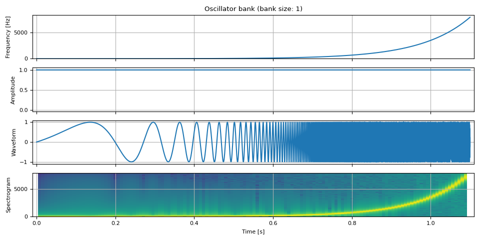
Let’s change the frequency over time. Here, we change the frequency from zero to the Nyquist frequency (half of the sample rate) in log-scale so that it is easy to see the change in waveform.

nyquist_freq = SAMPLE_RATE / 2
freq = torch.logspace(0, math.log(0.99 * nyquist_freq, 10), NUM_FRAMES).unsqueeze(-1)
amp = torch.ones((NUM_FRAMES, 1))

waveform = oscillator_bank(freq, amp, sample_rate=SAMPLE_RATE)

show(freq, amp, waveform, SAMPLE_RATE, vol=0.2)

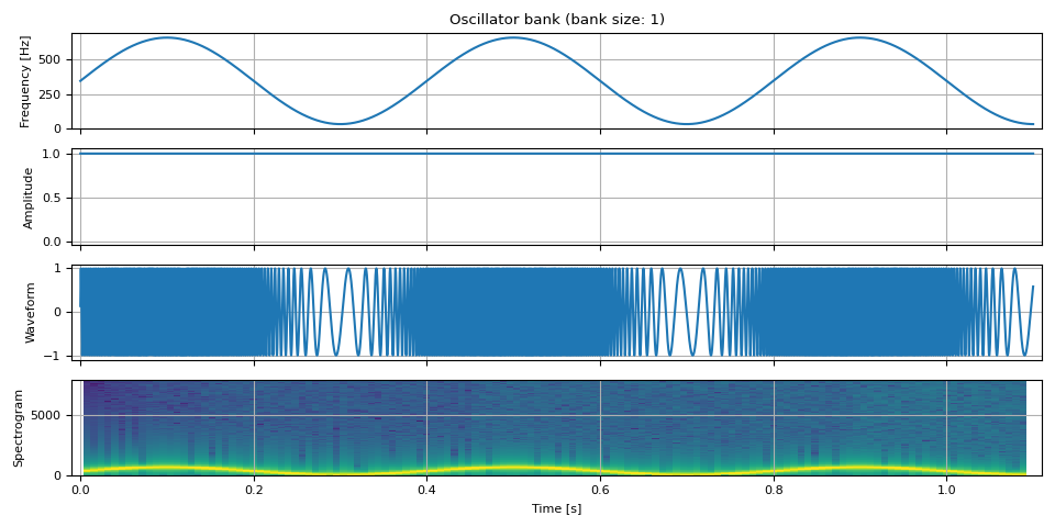
We can also oscillate frequency.

fm = 2.5  # rate at which the frequency oscillates
f_dev = 0.9 * F0  # the degree of frequency oscillation

freq = F0 + f_dev * torch.sin(torch.linspace(0, fm * PI2 * DURATION, NUM_FRAMES))
freq = freq.unsqueeze(-1)

amp = torch.ones((NUM_FRAMES, 1))

waveform = oscillator_bank(freq, amp, sample_rate=SAMPLE_RATE)

show(freq, amp, waveform, SAMPLE_RATE)

ADSR Envelope

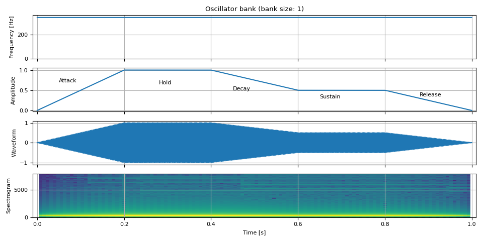
Next, we change the amplitude over time. A common technique to model amplitude is ADSR Envelope.

ADSR stands for Attack, Decay, Sustain, and Release.

• Attack is the time it takes to reach from zero to the top level.

• Decay is the time it takes from the top to reach sustain level.

• Sustain is the level at which the level stays constant.

• Release is the time it takes to drop to zero from sustain level.

There are many variants of ADSR model, additionally, some models have the following properties

• Hold: The time the level stays at the top level after attack.

• non-linear decay/release: The decay and release take non-linear change.

adsr_envelope supports hold and polynomial decay.

freq = torch.full((SAMPLE_RATE, 1), F0)
amp = adsr_envelope(
    SAMPLE_RATE,
    attack=0.2,
    hold=0.2,
    decay=0.2,
    sustain=0.5,
    release=0.2,
    n_decay=1,
)
amp = amp.unsqueeze(-1)

waveform = oscillator_bank(freq, amp, sample_rate=SAMPLE_RATE)

audio = show(freq, amp, waveform, SAMPLE_RATE)
ax = plt.gcf().axes[1]
ax.annotate("Attack", xy=(0.05, 0.7))
ax.annotate("Hold", xy=(0.28, 0.65))
ax.annotate("Decay", xy=(0.45, 0.5))
ax.annotate("Sustain", xy=(0.65, 0.3))
ax.annotate("Release", xy=(0.88, 0.35))
audio

Now let’s look into some examples of how ADSR envelope can be used to create different sounds.

The following examples are inspired by this article.

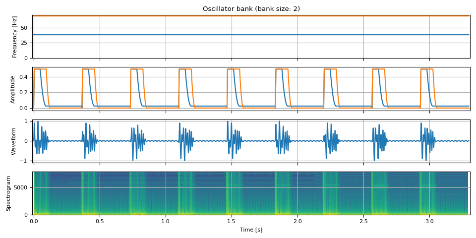
Drum Beats

unit = NUM_FRAMES // 3
repeat = 9

freq = torch.empty((unit * repeat, 2))
freq[:, 0] = F0 / 9
freq[:, 1] = F0 / 5

amp = torch.stack(
    (
        adsr_envelope(unit, attack=0.01, hold=0.125, decay=0.12, sustain=0.05, release=0),
        adsr_envelope(unit, attack=0.01, hold=0.25, decay=0.08, sustain=0, release=0),
    ),
    dim=-1,
)
amp = amp.repeat(repeat, 1) / 2

bass = oscillator_bank(freq, amp, sample_rate=SAMPLE_RATE)

show(freq, amp, bass, SAMPLE_RATE, vol=0.5)

Pluck

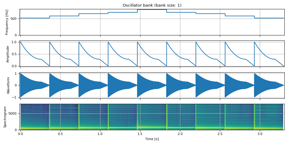
tones = [
    513.74,  # do
    576.65,  # re
    647.27,  # mi
    685.76,  # fa
    769.74,  # so
    685.76,  # fa
    647.27,  # mi
    576.65,  # re
    513.74,  # do
]

freq = torch.cat([torch.full((unit, 1), tone) for tone in tones], dim=0)
amp = adsr_envelope(unit, attack=0, decay=0.7, sustain=0.28, release=0.29)
amp = amp.repeat(9).unsqueeze(-1)

doremi = oscillator_bank(freq, amp, sample_rate=SAMPLE_RATE)

show(freq, amp, doremi, SAMPLE_RATE)

Riser

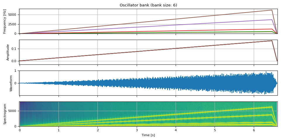
env = adsr_envelope(NUM_FRAMES * 6, attack=0.98, decay=0.0, sustain=1, release=0.02)

tones = [
    484.90,  # B4
    513.74,  # C5
    576.65,  # D5
    1221.88,  # D#6/Eb6
    3661.50,  # A#7/Bb7
    6157.89,  # G8
]
freq = torch.stack([f * env for f in tones], dim=-1)

amp = env.unsqueeze(-1).expand(freq.shape) / len(tones)

waveform = oscillator_bank(freq, amp, sample_rate=SAMPLE_RATE)

show(freq, amp, waveform, SAMPLE_RATE)

References

• https://www.edmprod.com/adsr-envelopes/

• https://pages.mtu.edu/~suits/notefreq432.html

• https://alijamieson.co.uk/2021/12/19/forgive-me-lord-for-i-have-synth-a-guide-to-subtractive-synthesis/