Note
Click here to download the full example code
Subtractive synthesis
Author: Moto Hira
This tutorial is the continuation of Filter Design Tutorial.
This tutorial shows how to perform subtractive synthesis with TorchAudio’s DSP functions.
Subtractive synthesis creates timbre by applying filters to source waveform.
Warning
This tutorial requires prototype DSP features, which are available in nightly builds.
Please refer to https://pytorch.org/get-started/locally for instructions for installing a nightly build.
import torch
import torchaudio

print(torch.__version__)
print(torchaudio.__version__)
2.2.0
2.2.0
Overview
try:
    from torchaudio.prototype.functional import filter_waveform, frequency_impulse_response, sinc_impulse_response
except ModuleNotFoundError:
    print(
        "Failed to import prototype DSP features. "
        "Please install torchaudio nightly builds. "
        "Please refer to https://pytorch.org/get-started/locally "
        "for instructions to install a nightly build."
    )
    raise

import matplotlib.pyplot as plt
from IPython.display import Audio
Filtered Noise
Subtractive synthesis starts with a waveform and applies filters to some frequency components.
For the first example of subtractive synthesis, we apply time-varying low pass filter to white noise.
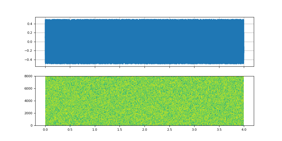
First, we create a white noise.
SAMPLE_RATE = 16_000
duration = 4
num_frames = int(duration * SAMPLE_RATE)

noise = torch.rand((num_frames,)) - 0.5
def plot_input():
    fig, axes = plt.subplots(2, 1, sharex=True)
    t = torch.linspace(0, duration, num_frames)
    axes[0].plot(t, noise)
    axes[0].grid(True)
    axes[1].specgram(noise, Fs=SAMPLE_RATE)
    Audio(noise, rate=SAMPLE_RATE)


plot_input()
Windowed-sinc filter
Sweeping cutoff frequency
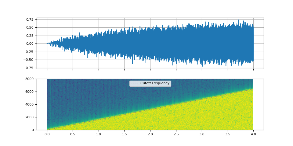
We use sinc_impulse_response() to
create series of low pass filters, while changing the cut-off
frequency from zero to Nyquist frequency.
num_filters = 64 * duration
window_size = 2049

f_cutoff = torch.linspace(0.0, 0.8, num_filters)
kernel = sinc_impulse_response(f_cutoff, window_size)
To apply time-varying filter, we use
filter_waveform()
Let’s look at the spectrogram of the resulting audio and listen to it.
def plot_sinc_ir(waveform, cutoff, sample_rate, vol=0.2):
    num_frames = waveform.size(0)
    duration = num_frames / sample_rate
    num_cutoff = cutoff.size(0)
    nyquist = sample_rate / 2

    _, axes = plt.subplots(2, 1, sharex=True)
    t = torch.linspace(0, duration, num_frames)
    axes[0].plot(t, waveform)
    axes[0].grid(True)
    axes[1].specgram(waveform, Fs=sample_rate, scale="dB")
    t = torch.linspace(0, duration, num_cutoff)
    axes[1].plot(t, cutoff * nyquist, color="gray", linewidth=0.8, label="Cutoff Frequency", linestyle="--")
    axes[1].legend(loc="upper center")
    axes[1].set_ylim([0, nyquist])
    waveform /= waveform.abs().max()
    return Audio(vol * waveform, rate=sample_rate, normalize=False)
plot_sinc_ir(filtered, f_cutoff, SAMPLE_RATE)
Oscillating cutoff frequency
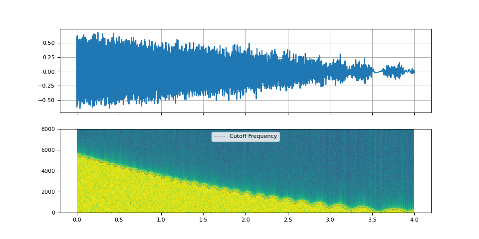
By oscillating the cutoff frequency, we can emulate an effect of Low-frequency oscillation (LFO).
PI2 = torch.pi * 2
num_filters = 90 * duration

f_lfo = torch.linspace(0.9, 0.1, num_filters)
f_cutoff_osci = torch.linspace(0.01, 0.03, num_filters) * torch.sin(torch.cumsum(f_lfo, dim=0))
f_cutoff_base = torch.linspace(0.8, 0.03, num_filters) ** 1.7
f_cutoff = f_cutoff_base + f_cutoff_osci
plot_sinc_ir(filtered, f_cutoff, SAMPLE_RATE)
Wah-wah effects
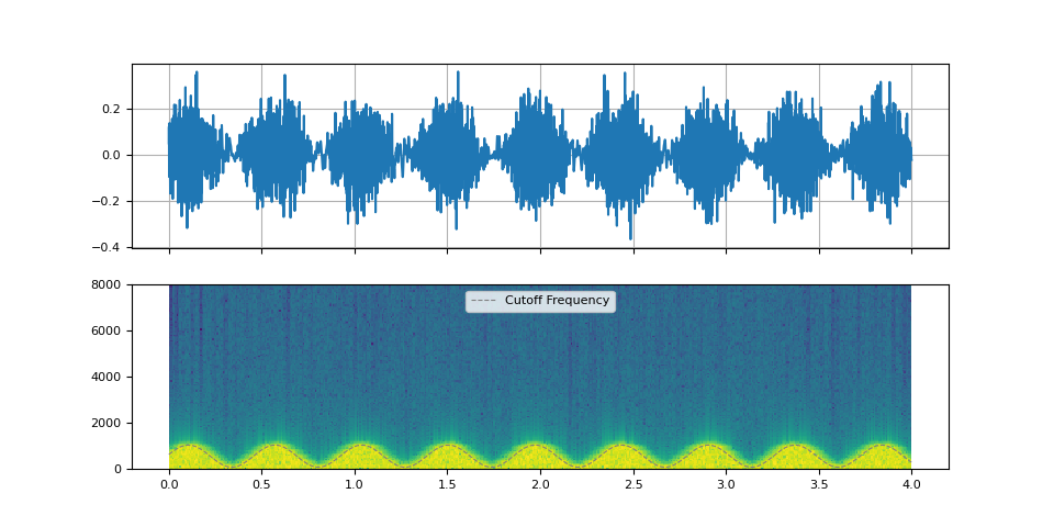
Wah-wah effects are applications of low-pass filter or band-pass filter. They change the cut-off freuqnecy or Q-factor quickly.
f_lfo = torch.linspace(0.15, 0.15, num_filters)
f_cutoff = 0.07 + 0.06 * torch.sin(torch.cumsum(f_lfo, dim=0))
plot_sinc_ir(filtered, f_cutoff, SAMPLE_RATE)
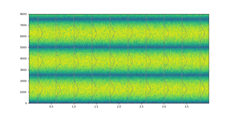
Arbitrary frequence response
By using
frequency_impulse_response(),
one can directly control the power distribution over frequency.
magnitudes = torch.sin(torch.linspace(0, 10, 64)) ** 4.0
kernel = frequency_impulse_response(magnitudes)
filtered = filter_waveform(noise, kernel.unsqueeze(0))
def plot_waveform(magnitudes, filtered, sample_rate):
    nyquist = sample_rate / 2
    num_samples = filtered.size(-1)
    duration = num_samples / sample_rate

    # Re-organize magnitudes for overlay
    N = 10  # number of overlays
    interval = torch.linspace(0.05, 0.95, N)
    offsets = duration * interval
    # Select N magnitudes for overlays
    mags = torch.stack(
        [magnitudes for _ in range(N)]
        if magnitudes.ndim == 1
        else [magnitudes[int(i * magnitudes.size(0))] for i in interval]
    )
    mag_x = offsets.unsqueeze(-1) + 0.1 * mags
    mag_y = torch.linspace(0, nyquist, magnitudes.size(-1)).tile((N, 1))

    _, ax = plt.subplots(1, 1, sharex=True)
    ax.vlines(offsets, 0, nyquist, color="gray", linestyle="--", linewidth=0.8)
    ax.plot(mag_x.T.numpy(), mag_y.T.numpy(), color="gray", linewidth=0.8)
    ax.specgram(filtered, Fs=sample_rate)
    return Audio(filtered, rate=sample_rate)
plot_waveform(magnitudes, filtered, SAMPLE_RATE)
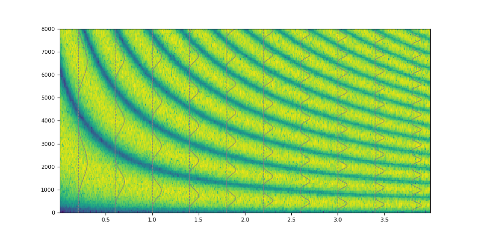
It is also possible to make a non-stationary filter.
magnitudes = torch.stack([torch.linspace(0.0, w, 1000) for w in torch.linspace(4.0, 40.0, 250)])
magnitudes = torch.sin(magnitudes) ** 4.0
kernel = frequency_impulse_response(magnitudes)
filtered = filter_waveform(noise, kernel)
plot_waveform(magnitudes, filtered, SAMPLE_RATE)
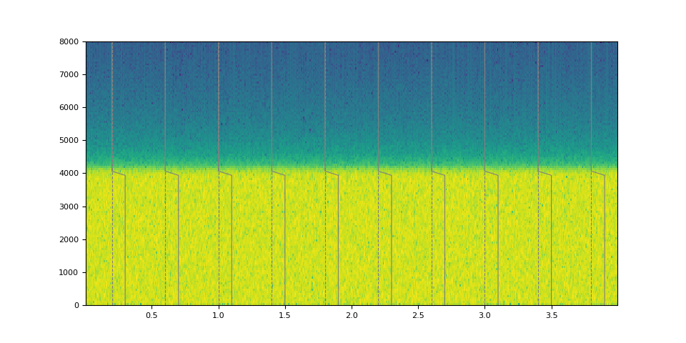
Of course it is also possible to emulate simple low pass filter.
magnitudes = torch.concat([torch.ones((32,)), torch.zeros((32,))])
kernel = frequency_impulse_response(magnitudes)
filtered = filter_waveform(noise, kernel.unsqueeze(0))
plot_waveform(magnitudes, filtered, SAMPLE_RATE)
References
Total running time of the script: ( 0 minutes 7.629 seconds)


