This post is the third part of a multi-series blog focused on how to accelerate generative AI models with pure, native PyTorch. We are excited to share a breadth of newly released PyTorch performance features alongside practical examples to see how far we can push PyTorch native performance. In part one, we showed how to accelerate Segment Anything over 8x using only pure, native PyTorch. In part two, we showed how to accelerate Llama-7B by almost 10x using only native PyTorch optimizations. In this blog, we’ll focus on speeding up text-to-image diffusion models by upto 3x.
We will leverage an array of optimizations including:
- Running with the bfloat16 precision
- scaled_dot_product_attention (SPDA)
- torch.compile
- Combining q,k,v projections for attention computation
- Dynamic int8 quantization
We will primarily focus on Stable Diffusion XL (SDXL), demonstrating a latency improvement of 3x. These techniques are PyTorch-native, which means you don’t have to rely on any third-party libraries or any C++ code to take advantage of them.
Enabling these optimizations with the 🤗Diffusers library takes just a few lines of code. If you’re already feeling excited and cannot wait to jump to the code, check out the accompanying repository here: https://github.com/huggingface/diffusion-fast.
(The discussed techniques are not SDXL-specific and can be used to speed up other text-to-image diffusion systems, as shown later.)
Below, you can find some blog posts on similar topics:
- Accelerated Diffusers with PyTorch 2.0
- Exploring simple optimizations for SDXL
- Accelerated Generative Diffusion Models with PyTorch 2
Setup
We will demonstrate the optimizations and their respective speed-up gains using the 🤗Diffusers library. Apart from that, we will make use of the following PyTorch-native libraries and environments:
- Torch nightly (to benefit from the fastest kernels for efficient attention; 2.3.0.dev20231218+cu121)
- 🤗 PEFT (version: 0.7.1)
- torchao (commit SHA: 54bcd5a10d0abbe7b0c045052029257099f83fd9)
- CUDA 12.1
For an easier reproduction environment, you can also refer to this Dockerfile. The benchmarking numbers presented in this post come from a 400W 80GB A100 GPU (with its clock rate set to its maximum capacity).
Since we use an A100 GPU (Ampere architecture) here, we can specify torch.set_float32_matmul_precision("high") to benefit from the TF32 precision format.
Run inference using a reduced precision
Running SDXL in Diffusers just takes a few lines of code:
from diffusers import StableDiffusionXLPipeline

## Load the pipeline in full-precision and place its model components on CUDA.
pipe = StableDiffusionXLPipeline.from_pretrained("stabilityai/stable-diffusion-xl-base-1.0").to("cuda")

## Run the attention ops without efficiency.
pipe.unet.set_default_attn_processor()
pipe.vae.set_default_attn_processor()

prompt = "Astronaut in a jungle, cold color palette, muted colors, detailed, 8k"
image = pipe(prompt, num_inference_steps=30).images[0]
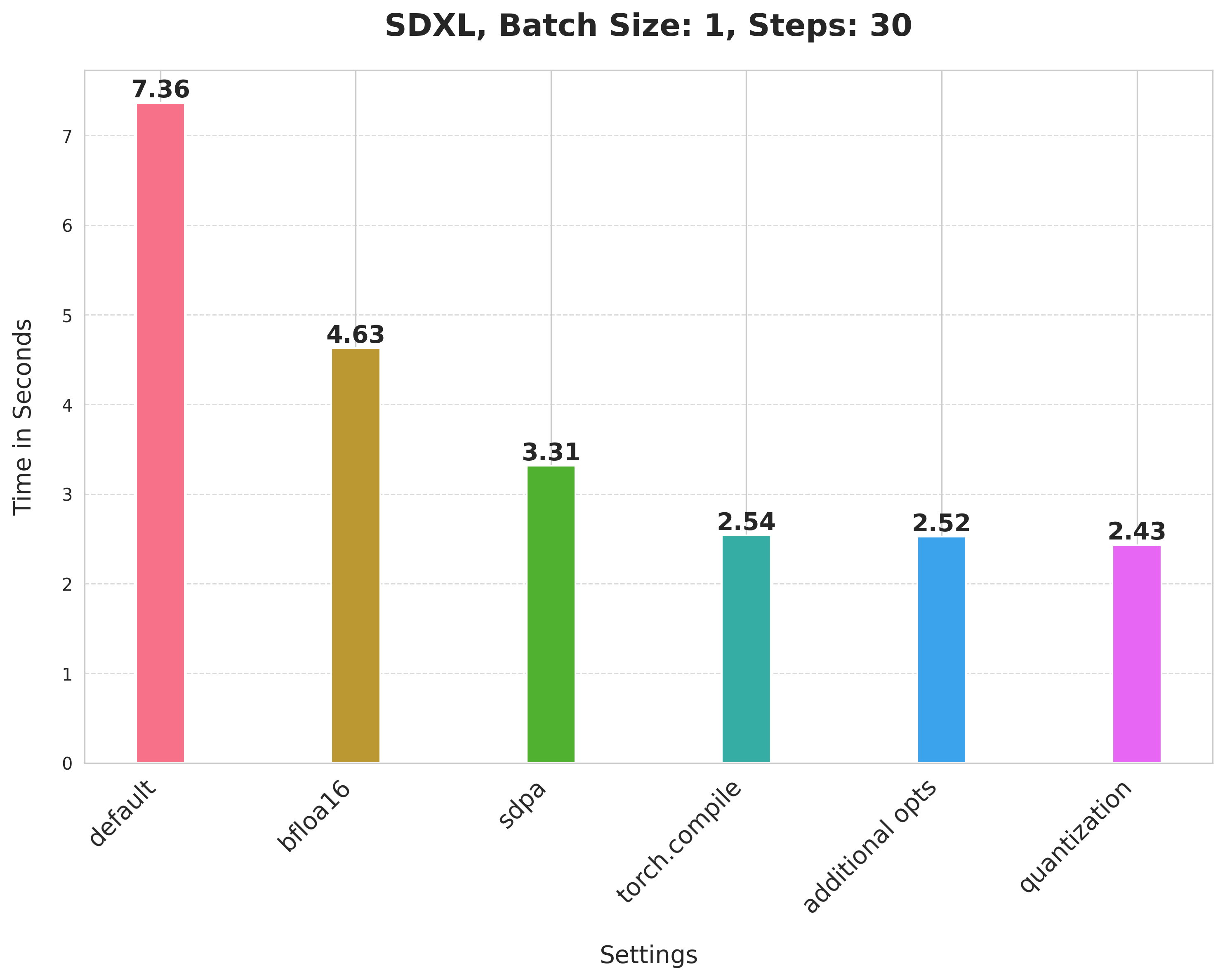
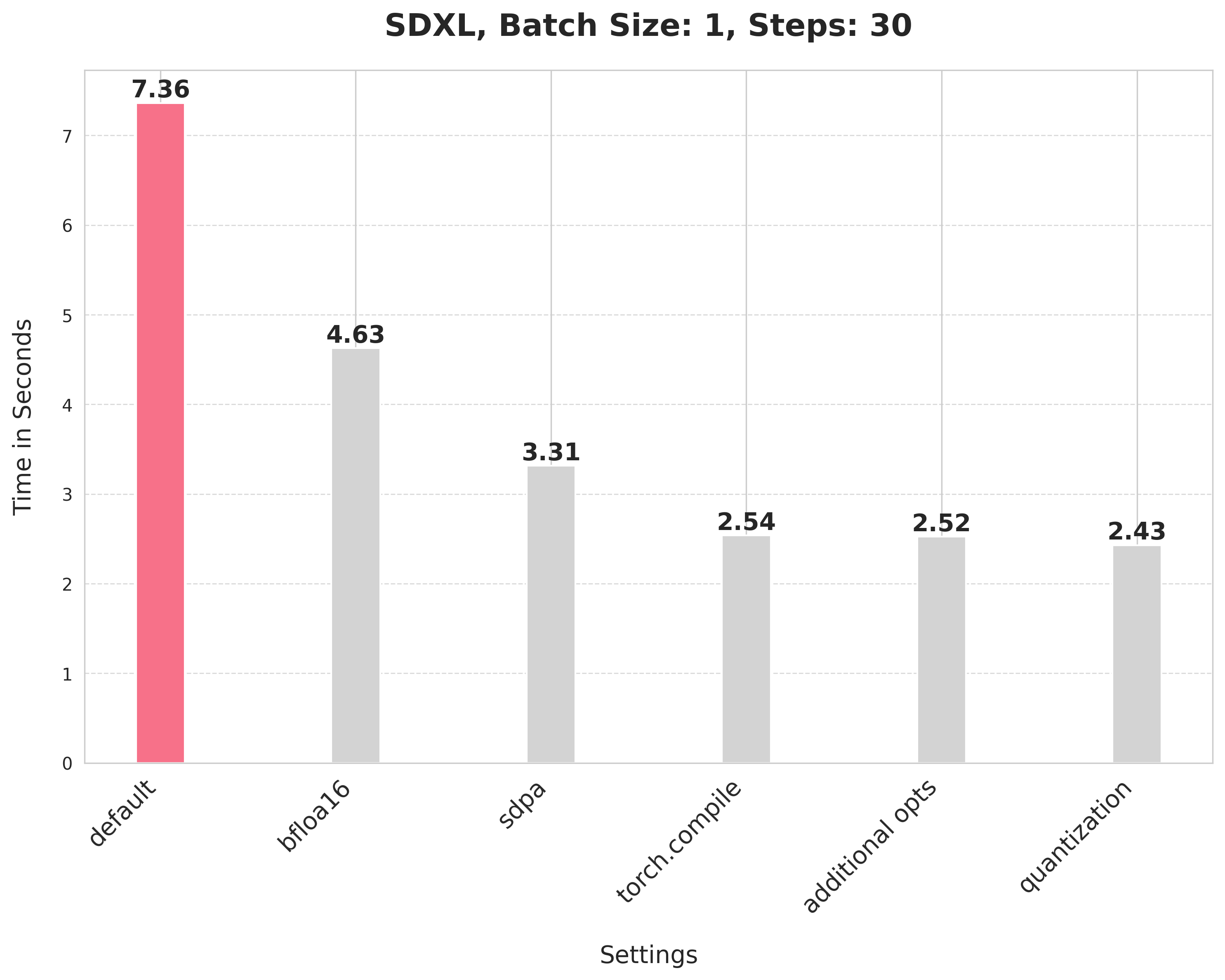
But this isn’t very practical as it takes 7.36 seconds to generate a single image with 30 steps. This is our baseline which we will try to optimize one step at a time.
Here, we’re running the pipeline with the full precision. We can immediately cut down the inference time by using a reduced precision such as bfloat16. Besides, modern GPUs come with dedicated cores for running accelerated computation benefiting from reduced precision. To run the computations of the pipeline in the bfloat16 precision, we just need to specify the data type while initializing the pipeline:
from diffusers import StableDiffusionXLPipeline

pipe = StableDiffusionXLPipeline.from_pretrained(
	"stabilityai/stable-diffusion-xl-base-1.0", torch_dtype=torch.bfloat16
).to("cuda")

## Run the attention ops without efficiency.
pipe.unet.set_default_attn_processor()
pipe.vae.set_default_attn_processor()
prompt = "Astronaut in a jungle, cold color palette, muted colors, detailed, 8k"
image = pipe(prompt, num_inference_steps=30).images[0]
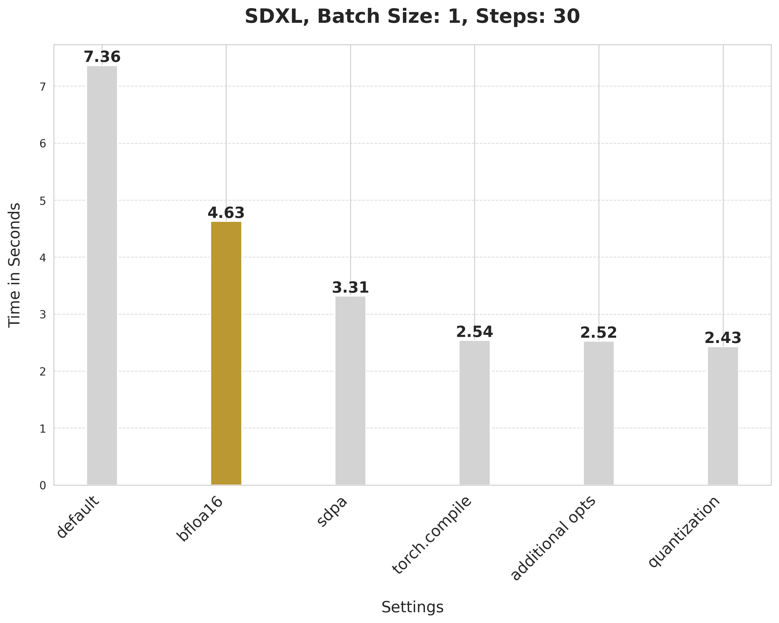
By using a reduced precision, we’re able to cut down the inference latency from 7.36 seconds to 4.63 seconds.
Some notes on the use of bfloat16
- Using a reduced numerical precision (such as float16, bfloat16) to run inference doesn’t affect the generation quality but significantly improves latency.
- The benefits of using the bfloat16 numerical precision as compared to float16 are hardware-dependent. Modern generations of GPUs tend to favor bfloat16.
- Furthermore, in our experiments, we bfloat16 to be much more resilient when used with quantization in comparison to float16.
(We later ran the experiments in float16 and found out that the recent versions of torchao do not incur numerical problems from float16.)
Use SDPA for performing attention computations
By default, Diffusers uses scaled_dot_product_attention (SDPA) for performing attention-related computations when using PyTorch 2. SDPA provides faster and more efficient kernels to run intensive attention-related operations. To run the pipeline SDPA, we simply don’t set any attention processor like so:
from diffusers import StableDiffusionXLPipeline

pipe = StableDiffusionXLPipeline.from_pretrained(
	"stabilityai/stable-diffusion-xl-base-1.0", torch_dtype=torch.bfloat16
).to("cuda")

prompt = "Astronaut in a jungle, cold color palette, muted colors, detailed, 8k"
image = pipe(prompt, num_inference_steps=30).images[0]
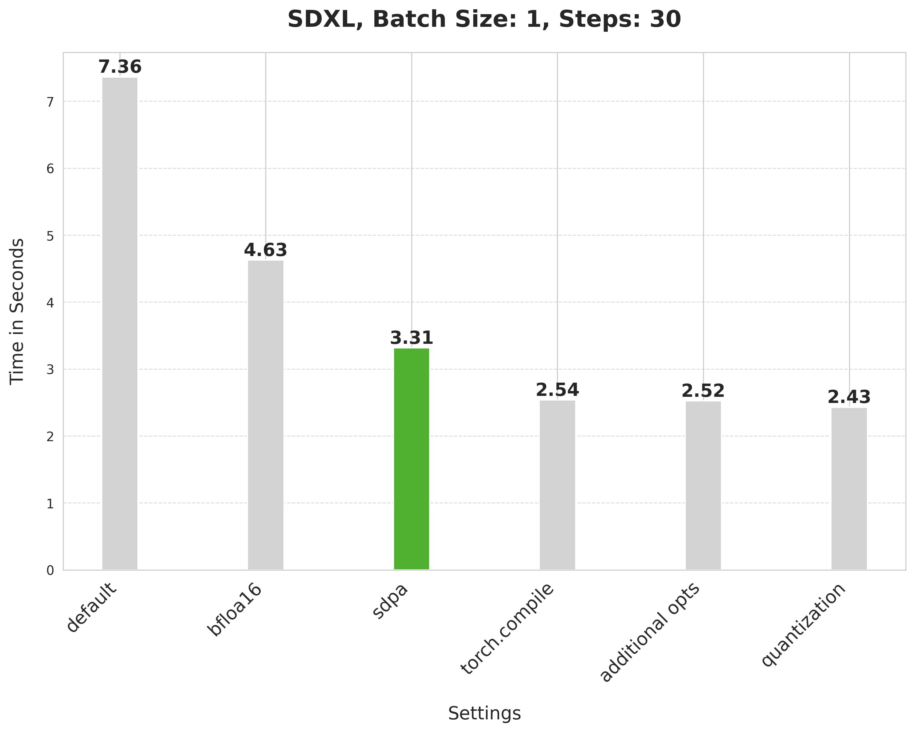
SDPA gives a nice boost from 4.63 seconds to 3.31 seconds.
Compiling the UNet and VAE
We can ask PyTorch to perform some low-level optimizations (such as operator fusion and launching faster kernels with CUDA graphs) by using torch.compile. For the StableDiffusionXLPipeline, we compile the denoiser (UNet) and the VAE:
from diffusers import StableDiffusionXLPipeline
import torch

pipe = StableDiffusionXLPipeline.from_pretrained(
    "stabilityai/stable-diffusion-xl-base-1.0", torch_dtype=torch.bfloat16
).to("cuda")

## Compile the UNet and VAE.
pipe.unet = torch.compile(pipe.unet, mode="max-autotune", fullgraph=True)
pipe.vae.decode = torch.compile(pipe.vae.decode, mode="max-autotune", fullgraph=True)

prompt = "Astronaut in a jungle, cold color palette, muted colors, detailed, 8k"

## First call to `pipe` will be slow, subsequent ones will be faster.
image = pipe(prompt, num_inference_steps=30).images[0]
Using SDPA attention and compiling both the UNet and VAE reduces the latency from 3.31 seconds to 2.54 seconds.
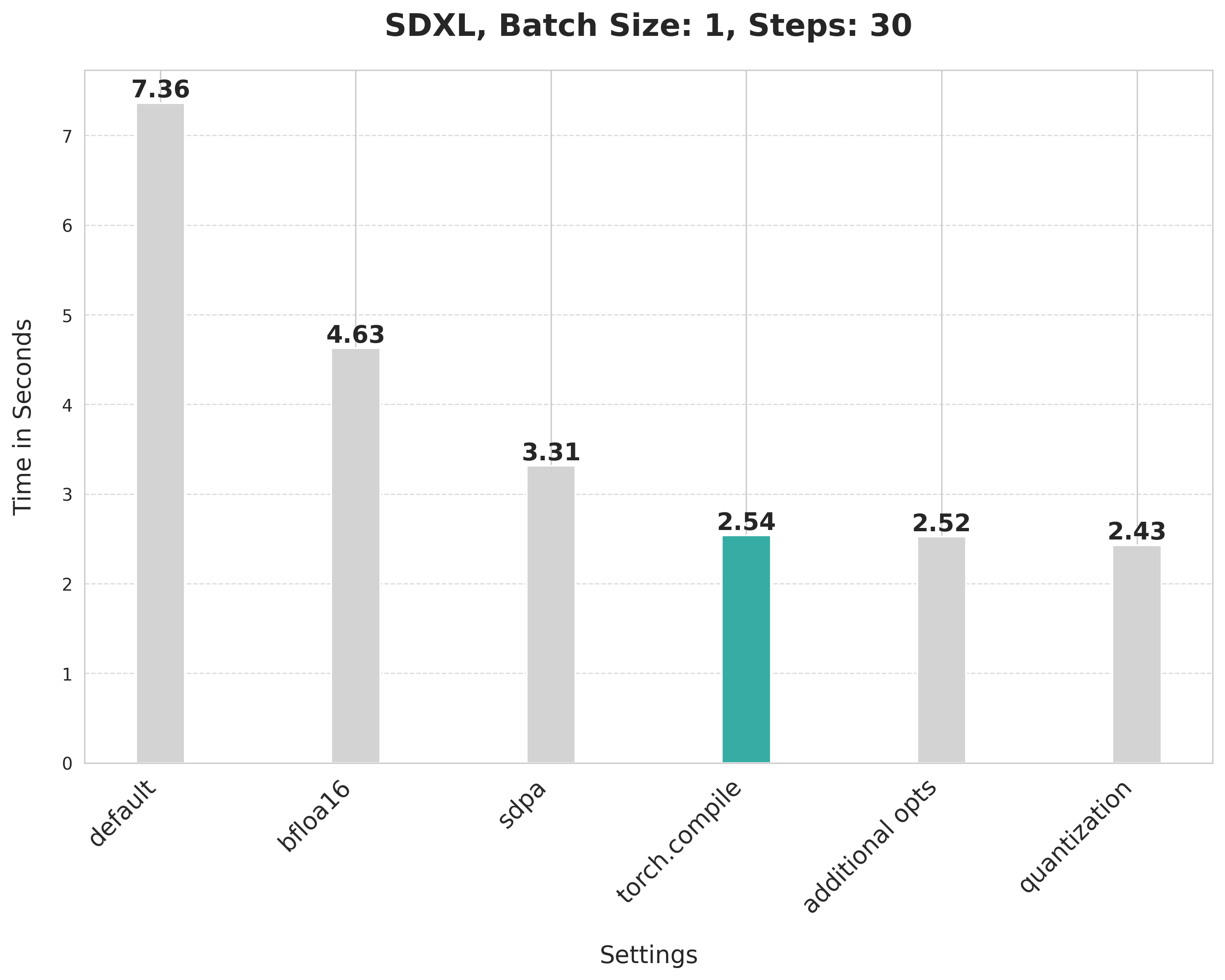
Notes on torch.compile
torch.compile offers different backends and modes. As we’re aiming for maximum inference speed, we opt for the inductor backend using the “max-autotune”. “max-autotune” uses CUDA graphs and optimizes the compilation graph specifically for latency. Using CUDA graphs greatly reduces the overhead of launching GPU operations. It saves time by using a mechanism to launch multiple GPU operations through a single CPU operation.
Specifying fullgraph to be True ensures that there are no graph breaks in the underlying model, ensuring the fullest potential of torch.compile. In our case, the following compiler flags were also important to be explicitly set:
torch._inductor.config.conv_1x1_as_mm = True
torch._inductor.config.coordinate_descent_tuning = True
torch._inductor.config.epilogue_fusion = False
torch._inductor.config.coordinate_descent_check_all_directions = True
For the full list of compiler flags, refer to this file.
We also change the memory layout of the UNet and the VAE to “channels_last” when compiling them to ensure maximum speed:
pipe.unet.to(memory_format=torch.channels_last)
pipe.vae.to(memory_format=torch.channels_last)
In the next section, we’ll show how to improve the latency even further.
Additional optimizations
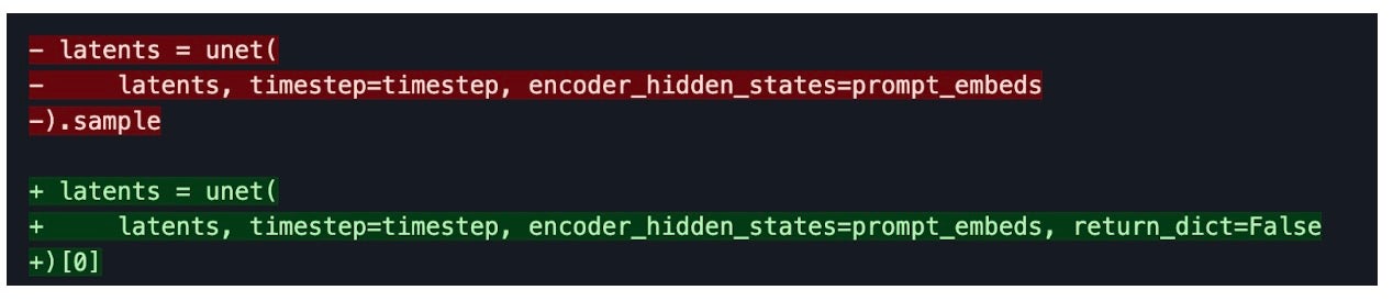
No graph breaks during torch.compile
Ensuring that the underlying model/method can be fully compiled is crucial for performance (torch.compile with fullgraph=True). This means having no graph breaks. We did this for the UNet and VAE by changing how we access the returning variables. Consider the following example:
Getting rid of GPU syncs after compilation
During the iterative reverse diffusion process, we call step() on the scheduler each time after the denoiser predicts the less noisy latent embeddings. Inside step(), the sigmas variable is indexed. If the sigmas array is placed on the GPU, indexing causes a communication sync between the CPU and GPU. This causes a latency, and it becomes more evident when the denoiser has already been compiled.
But if the sigmas array always stays on the CPU (refer to this line), this sync doesn’t take place, hence improved latency. In general, any CPU <-> GPU communication sync should be none or be kept to a bare minimum as it can impact inference latency.
Using combined projections for attention ops
Both the UNet and the VAE used in SDXL make use of Transformer-like blocks. A Transformer block consists of attention blocks and feed-forward blocks.
In an attention block, the input is projected into three sub-spaces using three different projection matrices – Q, K, and V. In the naive implementation, these projections are performed separately on the input. But we can horizontally combine the projection matrices into a single matrix and perform the projection in one shot. This increases the size of the matmuls of the input projections and improves the impact of quantization (to be discussed next).
Enabling this kind of computation in Diffusers just takes a single line of code:
pipe.fuse_qkv_projections()
This will make the attention operations for both the UNet and the VAE take advantage of the combined projections. For the cross-attention layers, we only combine the key and value matrices. To learn more, you can refer to the official documentation here. It’s worth noting that we leverage PyTorch’s scaled_dot_product_attention here internally.
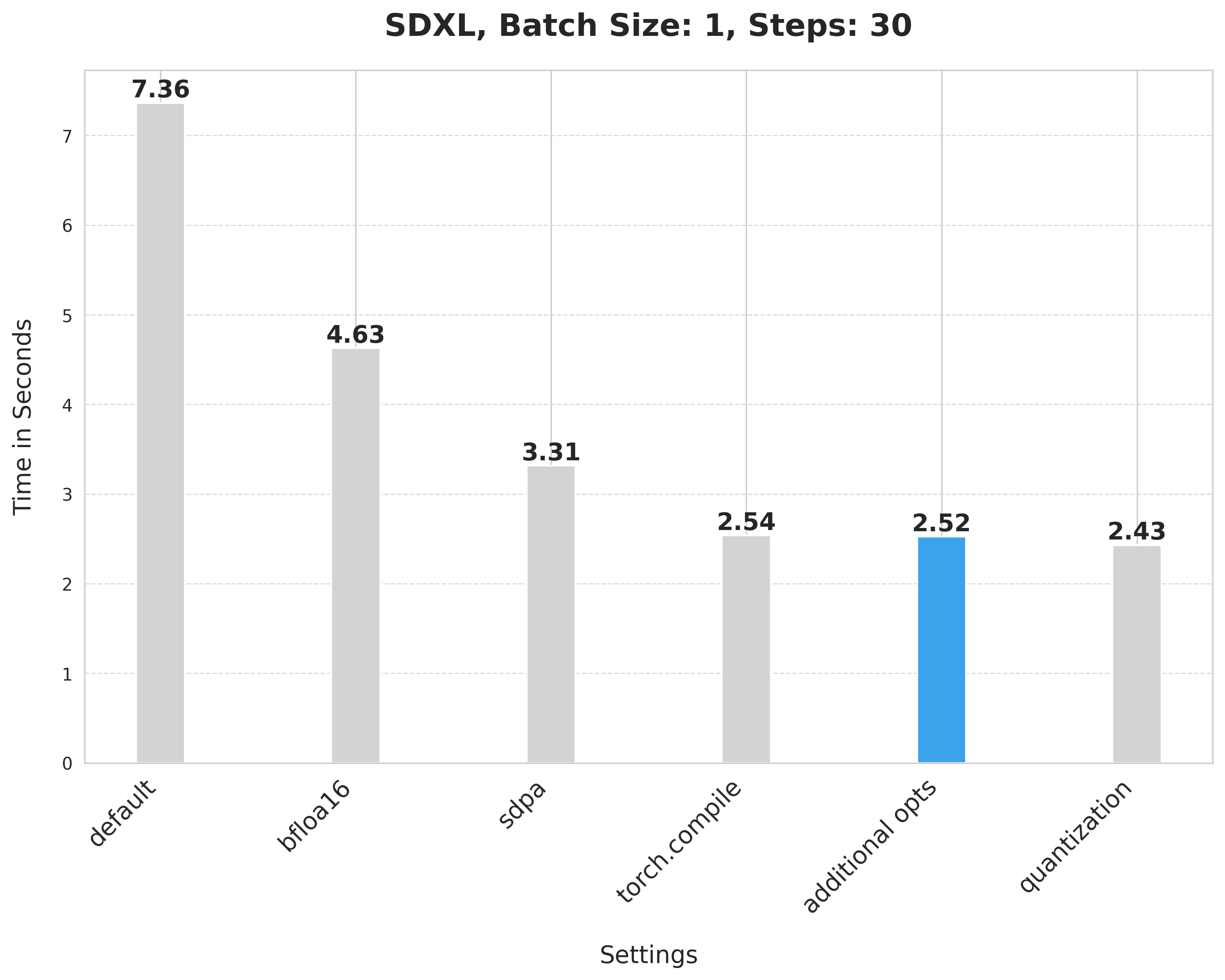
These additional techniques improved the inference latency from 2.54 seconds to 2.52 seconds.
Dynamic int8 quantization
We selectively apply dynamic int8 quantization to both the UNet and the VAE. This is because quantization adds additional conversion overhead to the model that is hopefully made up for by faster matmuls (dynamic quantization). If the matmuls are too small, these techniques may degrade performance.
Through experimentation, we found that certain linear layers in the UNet and the VAE don’t benefit from dynamic int8 quantization. You can check out the full code for filtering those layers here (referred to as dynamic_quant_filter_fn below).
We leverage the ultra-lightweight pure PyTorch library torchao to use its user-friendly APIs for quantization:
from torchao.quantization import apply_dynamic_quant

apply_dynamic_quant(pipe.unet, dynamic_quant_filter_fn)
apply_dynamic_quant(pipe.vae, dynamic_quant_filter_fn)
Since this quantization support is limited to linear layers only, we also turn suitable pointwise convolution layers into linear layers to maximize the benefit. We also specify the following compiler flags when using this option:
torch._inductor.config.force_fuse_int_mm_with_mul = True
torch._inductor.config.use_mixed_mm = True
To prevent any numerical issues stemming from quantization, we run everything in the bfloat16 format.
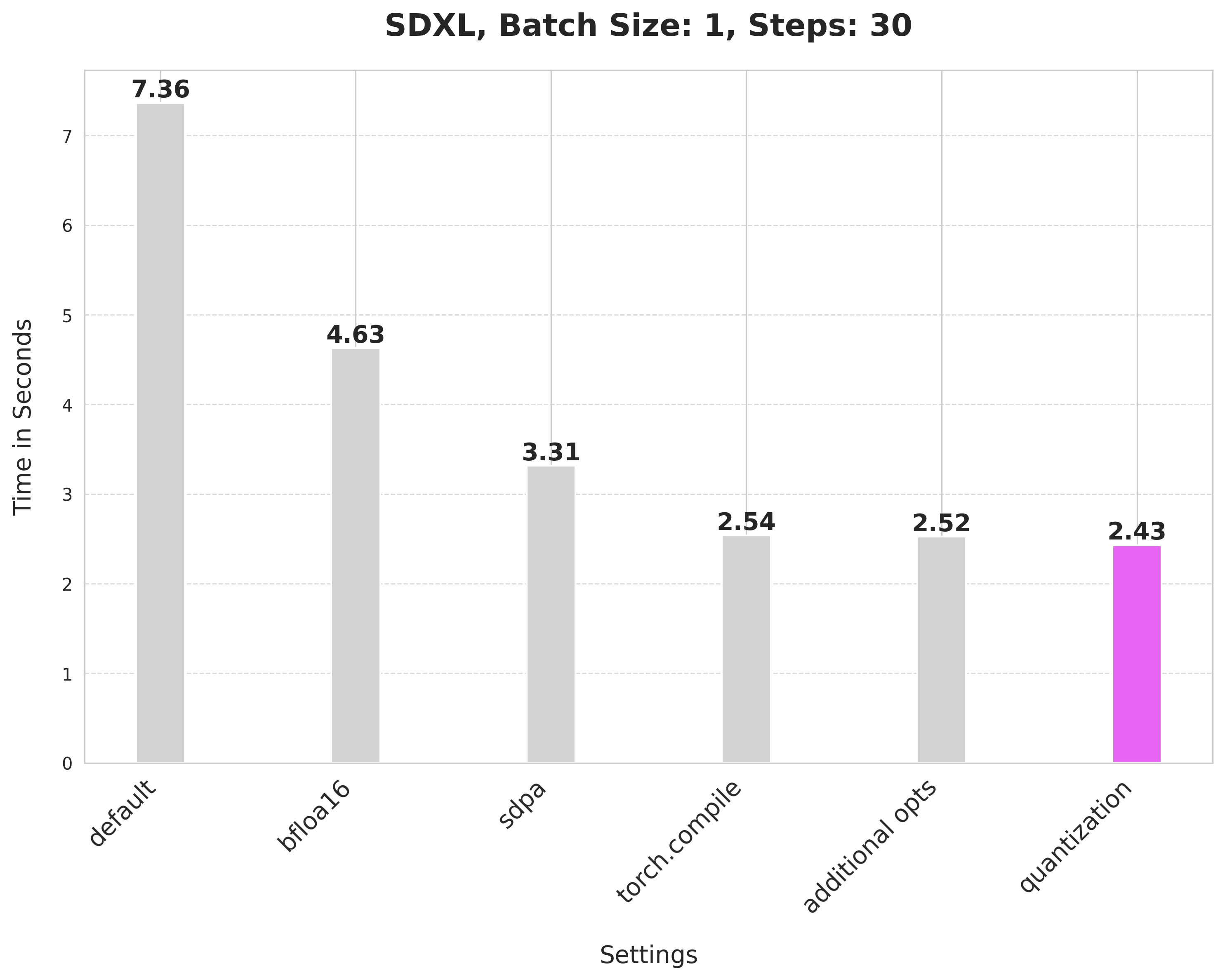
Applying quantization this way improved the latency from 2.52 seconds to 2.43 seconds.
Resources
We welcome you to check out the following codebases to reproduce these numbers and extend the techniques to other text-to-image diffusion systems as well:
- diffusion-fast (repository providing all the code to reproduce the numbers and plots above)
- torchao library
- Diffusers library
- PEFT library
Other links
- SDXL: Improving Latent Diffusion Models for High-Resolution Image Synthesis
- Fast diffusion documentation
Improvements in other pipelines
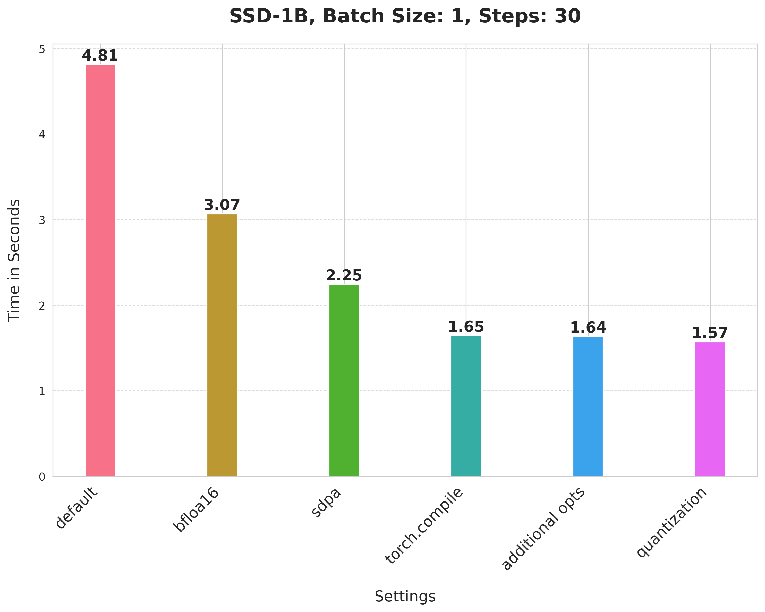
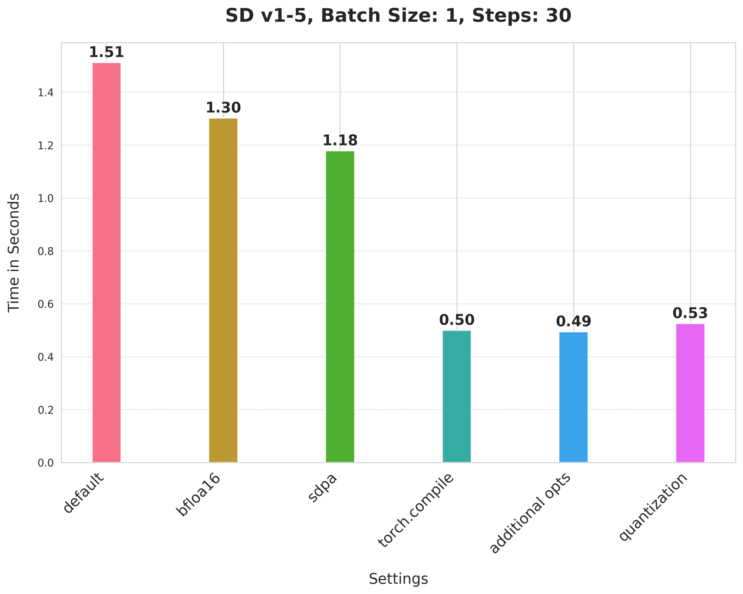
We applied these techniques to other pipelines to test the generality of our approach. Below are our findings:
SSD-1B
Stable Diffusion v1-5
PixArt-alpha/PixArt-XL-2-1024-MS
It’s worth noting that PixArt-Alpha uses a Transformer-based architecture as its denoiser for the reverse diffusion process instead of a UNet.
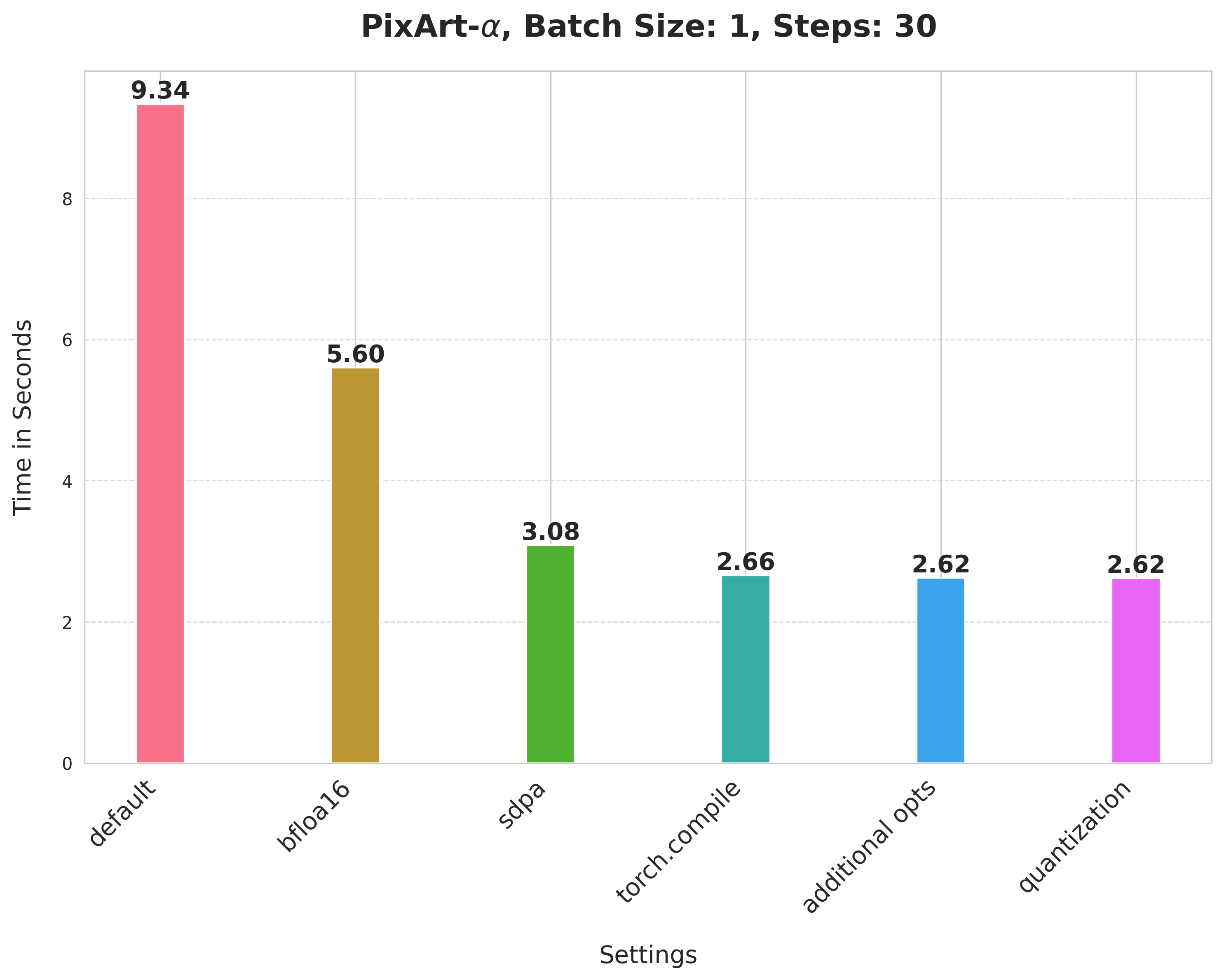
Note that for Stable Diffusion v1-5 and PixArt-Alpha, we didn’t explore the best shape combination criteria for applying dynamic int8 quantization. It might be possible to get better numbers with a better combination.
Collectively, the methods we presented offer substantial speedup over the baseline without degradation in the generation quality. Furthermore, we believe that these methods should complement other optimization methods popular in the community (such as DeepCache, Stable Fast, etc.).
Conclusion and next steps
In this post, we presented a basket of simple yet effective techniques that can help improve the inference latency of text-to-image Diffusion models in pure PyTorch. In summary:
- Using a reduced precision to perform our computations
- Scaled-dot product attention for running the attention blocks efficiently
- torch.compile with “max-autotune” to improve for latency
- Combining the different projections together for computing attention
- Dynamic int8 quantization
We believe there’s a lot to be explored in terms of how we apply quantization to a text-to-image diffusion system. We didn’t exhaustively explore which layers in the UNet and the VAE tend to benefit from dynamic quantization. There might be opportunities to further speed things up with a better combination of the layers being targeted for quantization.
We kept the text encoders of SDXL untouched other than just running them in bfloat16. Optimizing them might also lead to improvements in latency.
Acknowledgements
Thanks to Ollin Boer Bohan whose VAE was used throughout the benchmarking process as it is numerically more stable under reduced numerical precisions.
Thanks to Hugo Larcher from Hugging Face for helping with infrastructure.