An efficient decoding Grouped-Query Attention with low-precision KV cache
Introduction
Generative AI has taken the world by storm with its ability to generate content like humans. Many of these generative AI tools are powered by large language models (LLMs), like Meta Llama models and OpenAI’s ChatGPT. One of the main challenges of LLMs is supporting large “context lengths” (also known as “sequence lengths”). The context length refers to the number of tokens that the model uses to understand the input context and generate responses. Longer context lengths generally translate into higher precision and quality in the responses. However, long context lengths are compute and memory intensive. This is mainly due to the following reasons:
- The computational complexity of attention layers increases proportionally with the context length (the growth rate depends on the attention algorithm). As a result, when using long context lengths, the attention layers can become a bottleneck, particularly during the prefill phase where attentions are compute bound.
- The KV cache size grows linearly with the context length, thus, putting higher pressure on the memory requirement and consequently slowing down the already memory-bound attention decoding. Moreover, since the memory capacity is limited, the batch size reduces when the KV cache gets bigger, which generally results in a drop in throughput.
The computational complexity growth is difficult to solve compared to the other problem mentioned above. One way to address the KV cache size growth problem is to use low precision KV cache. From our experiments, group-wise INT4 quantization provides comparable results in terms of accuracy compared to BF16 KV cache during the decode phase in Meta Llama 2 inference. However, we did not observe any latency improvement, despite reading 4x lesser data in attention decoding layers. This means that the INT4 attention is 4x less efficient at utilizing precious HBM bandwidth than BF16 attention.
In this note, we discuss the CUDA optimizations that we applied to INT4 GQA (grouped-query attention – the attention layer that we use in the LLM inference phase) to improve its performance by up to 1.8x on the NVIDIA A100 GPU and 1.9x on the NVIDIA H100 GPU.
- The optimized CUDA INT4 GQA outperformed INT4 Flash-Decoding GQA (the best performing INT4 GQA that we used in the experiment mentioned above) by 1.4x-1.7x on A100 and 1.09x-1.3x on H100.
- The optimized CUDA INT4 GQA performs better than BF16 Flash-Decoding GQA by 1.5x-1.7x on A100 and 1.4x-1.7x on H100.
Background
GQA for LLM Inference
Grouped-Query Attention (GQA) is a variant of multi-head attention (MHA) where each KV cache head is shared across a group of query heads. Our LLM inference adopts GQA as an attention layer in both the prefill and decode phases in order to reduce the capacity requirement for the KV cache. We use multiple GPUs in inference where the KV cache and query heads are distributed across GPUs. Each GPU runs an attention layer with a single KV head and a group of Q heads. Therefore, when viewed from a single GPU perspective, the GQA component can also be described as MQA (Multi-Query Attention).
The simplified workflow of decoding GQA is illustrated in Figure 1. GQA takes three main inputs: input query (denoted Q), K cache (denoted K), and V cache (denoted V). Our current GQA inference uses BF16 for Q, K, and V.
Qis a 4D BF16 tensor of shape (B,1,HQ,D)Kis a 4D BF16 tensor of shape (B,Tmax,HKV,D)Vis a 4D BF16 tensor of shape (B,Tmax,HKV,D)
where
Bis the batch size (the number of input prompts)HQis the number of query headsHKVis the number of KV heads (HQmust be divisible byHKV)Tmaxis the maximum context lengthDis the head dimension (fixed to 128)
GQA is simply bmm(softmax(bmm(Q, KT) / sqrt(D)), V). This yields a single output tensor (denoted as O) which is a 4D BF16 tensor that has the same shape as Q. Note that matrix multiplications are performed using BF16, however, accumulation and softmax are carried out in FP32. We call this “BF16 GQA” as the KV cache is BF16.
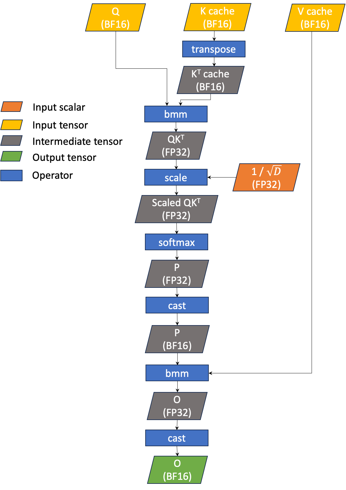
Figure 1 The simplified workflow of BF16 GQA for LLM inference
INT4 GQA
To further reduce the size of the KV cache, we explore the possibility of using INT4 for KV cache instead of BF16. We estimate the potential performance improvement by calculating the computational intensity (CI) of INT4 GQA and comparing it to that of BF16 GQA, as CI represents FLOPS per byte. We compute the CI for QKT and PV (as shown in Equation 1) as they take KV cache as an operand. Note that we disregard the Q load as it is negligible compared to the KV cache. We also ignore any intermediate data loads/stores that are not on global memory. Thus, the CI only takes into account the computation FLOPS and KV cache loads.
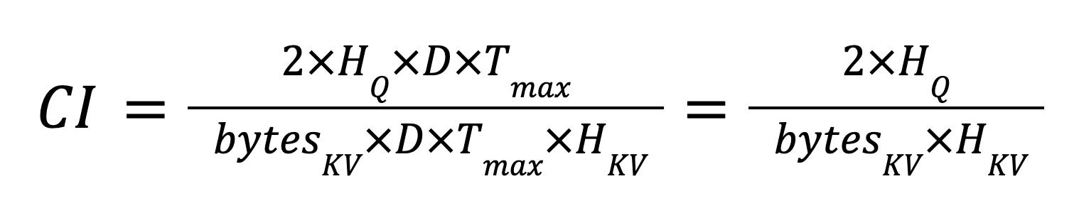
Equation (1)
Assuming that HQ = 8 and HKV = 1, CI for BF16 KV cache is 8 while CI for INT4 KV cache is 32. The CIs indicate that both BF16 and INT4 GQAs are memory bound (the peak CIs for BF16 tensor cores for A100 and H100 are 312 TF / 2 TB/s = 141 and 990 TF / 3.35 TB/s = 269; note that these TF numbers are without sparsity). Moreover, with INT4 KV cache, we should expect up to 4x performance improvement compared to BF16 GQA.
To enable INT4 KV cache support in GQA, we can dequantize the KV cache from INT4 to BF16 before passing it to the BF16 GQA operator. However, since KV cache is typically large, copying it from/to global memory can be costly. Moreover, decoding GQA is a memory bound operation (the memory unit is utilized much more heavily than the compute unit). Figure 2 shows the NCU profile of the FMHA CUTLASS BF16 GQA kernel in xFormers, which is one of the state of the art implementations of GQA. From the figure, it is obvious that memory is a bottleneck.
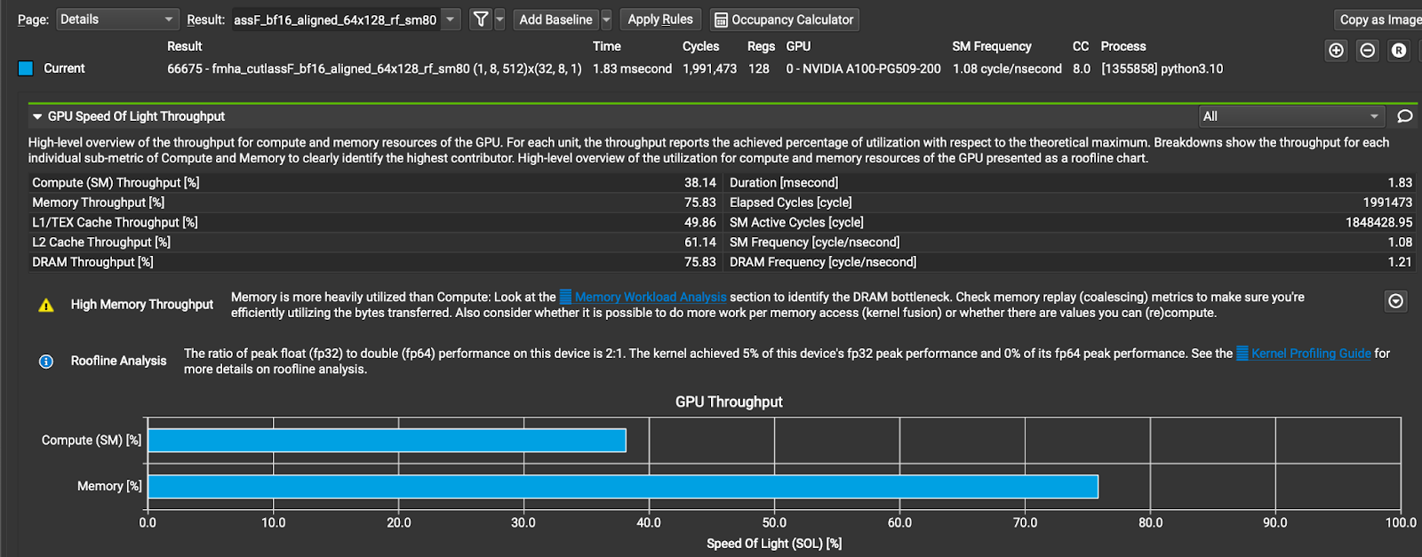
Figure 2 The NCU profile of the FMHA CUTLASS BF16 kernel in xFormers
A more efficient alternative is to fuse INT4 dequantization with the GQA operation (shown in Figure 3). In other words, having GQA read INT4 KV cache directly and perform the INT4 to BF16 conversion within the kernel. This change can potentially reduce the amount of global memory reads required for the KV cache, which could lead to a decrease in latency. We call this “INT4 GQA.”
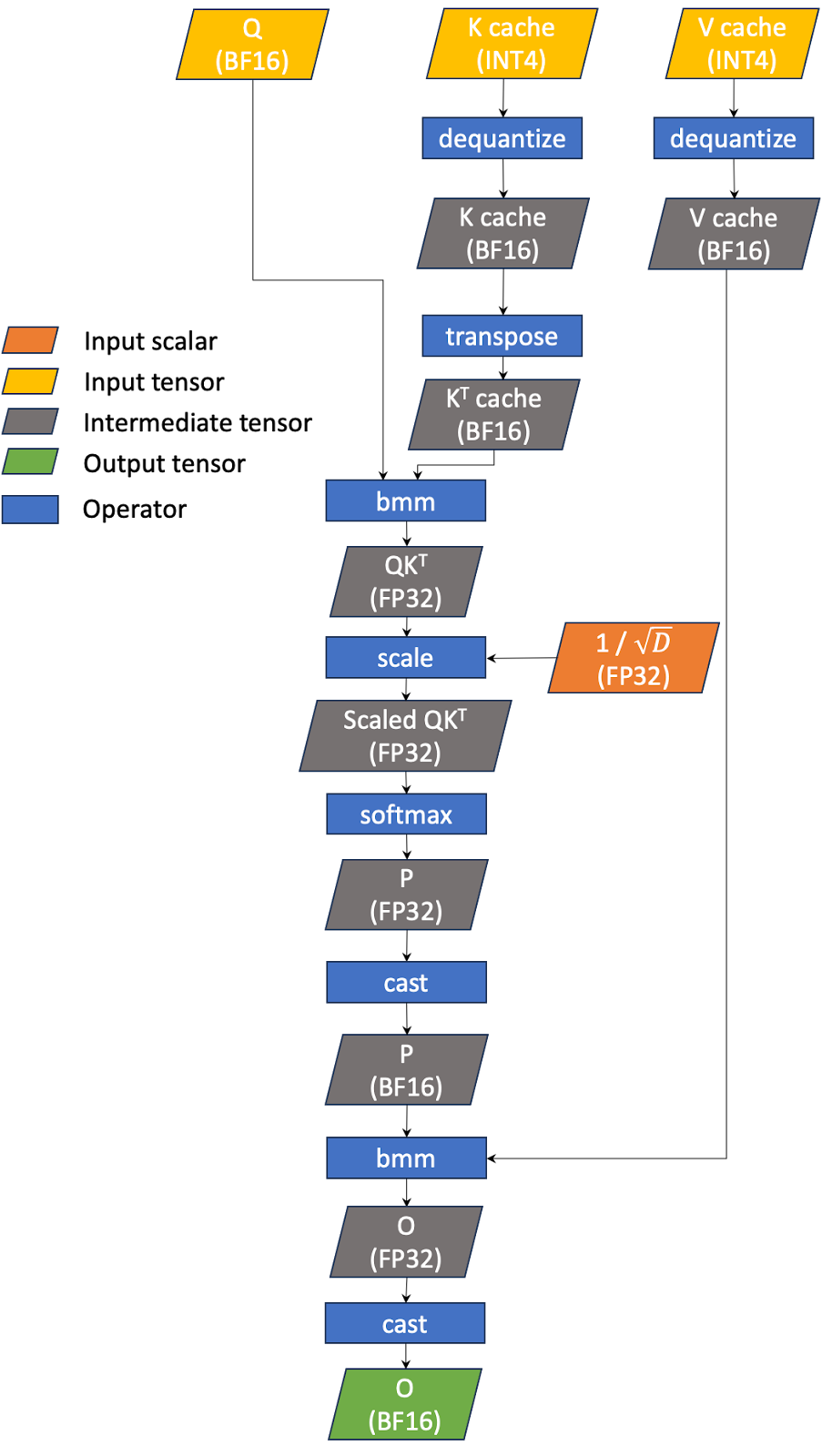
Figure 3 The workflow of fused INT4 GQA
We list the state of the art implementations of GQA in the table below along with their features in Table 1.
Table 1 State of the art GQA implementations
| Implementation | Denote | BF16 GQA | Fused INT4 GQA |
| Flash-Decoding (Triton implementation) | FD | Yes | Yes |
| Flash Attention (v2.3.3) | FA | Yes | No |
| CUDA baseline | CU | Yes | Yes |
All implementations, except for CU, support both split-K and non split-K. CU only has the split-K implementation. Only FA has a heuristic in the backend to determine whether to run the split-K or non split-K kernel. For other implementations, users must explicitly choose which version to run. In this note, we focus on long context lengths (in our experiments, we use a context length of 8192) and therefore opt for the split-K version wherever possible.
As the baseline, we measured the performance of the state of the art GQA implementations on NVIDIA A100 and H100 GPUs. The latency (time in microseconds) and achieved bandwidth (GB/s) are reported in Table 2. Note that we ran a range of split-Ks (from 2 to 128 splits) and reported the best performance for each implementation. For all experiments, we use a context length of 8192. For INT4 GQA, we used row-wise quantization (i.e., num quantized groups = 1).
Table 2 Baseline GQA performance
On A100
| Time (us) | BF16 GQA | INT4 GQA | ||||
| Batch size | FD | FA | CU | FD | FA | CU |
| 32 | 139 | 133 | 183 | 137 | – | 143 |
| 64 | 245 | 229 | 335 | 234 | – | 257 |
| 128 | 433 | 555 | 596 | 432 | – | 455 |
| 256 | 826 | 977 | 1127 | 815 | – | 866 |
| 512 | 1607 | 1670 | 2194 | 1581 | – | 1659 |
| Effective Bandwidth (GB/s) | BF16 GQA | INT4 GQA | ||||
| Batch size | FD | FA | CU | FD | FA | CU |
| 32 | 965 | 1012 | 736 | 262 | – | 250 |
| 64 | 1097 | 1175 | 802 | 305 | – | 278 |
| 128 | 1240 | 968 | 901 | 331 | – | 314 |
| 256 | 1301 | 1100 | 954 | 351 | – | 331 |
| 512 | 1338 | 1287 | 980 | 362 | – | 345 |
On H100
| Time (us) | BF16 GQA | INT4 GQA | ||||
| Batch size | FD | FA | CU | FD | FA | CU |
| 32 | 91 | 90 | 114 | 70 | – | 96 |
| 64 | 148 | 146 | 200 | 113 | – | 162 |
| 128 | 271 | 298 | 361 | 205 | – | 294 |
| 256 | 515 | 499 | 658 | 389 | – | 558 |
| 512 | 1000 | 1011 | 1260 | 756 | – | 1066 |
| Effective Bandwidth (GB/s) | BF16 GQA | INT4 GQA | ||||
| Batch size | FD | FA | CU | FD | FA | CU |
| 32 | 1481 | 1496 | 1178 | 511 | – | 371 |
| 64 | 1815 | 1840 | 1345 | 631 | – | 443 |
| 128 | 1982 | 1802 | 1487 | 699 | – | 487 |
| 256 | 2087 | 2156 | 1634 | 736 | – | 513 |
| 512 | 2150 | 2127 | 1706 | 757 | – | 537 |
First, let’s discuss the BF16 GQA performance: CU ranks last in terms of performance among all implementations. FD and FA have comparable performance. When the batch size is less than or equal to 64, FA utilizes the split-K kernel and performs slightly better than FD. However, when the batch size is greater than 64, FD performs better.
The same trend holds true for INT4 GQAs. However, we did not measure the performance of FA as it does not support INT4 KV cache. FD outperforms CU for all cases.
When comparing the latencies of FD between BF16 and INT4 GQAs, we find that they are almost identical. This suggests that INT4 GQA is highly inefficient, which can be further confirmed by the significantly lower achievable bandwidth for INT4 GQA compared to BF16 GQA. The same trend is also true when looking at the performance of CU.
CUDA with Tensor Cores INT4 GQA Implementation
In this section, we briefly describe our baseline implementation which is CUDA with tensor cores INT4 GQA (CU). Each thread block processes only one KV head and a group of query heads from one input prompt. Therefore, each thread block performs mm(softmax(mm(Q, KT) / sqrt(D)), V); notice that mm is being performed not bmm. Moreover, since this is a split-K implementation, tokens in the KV cache are split among different thread blocks. Note that each thread block contains 4 warps (each warp contains 32 threads for NVIDIA A100 and H100 GPUs). Work in each thread block is split among warps. Within each warp, we use the WMMA API to compute matrix multiplication on tensor cores. Figure 4 demonstrates the work partitioning in CU.
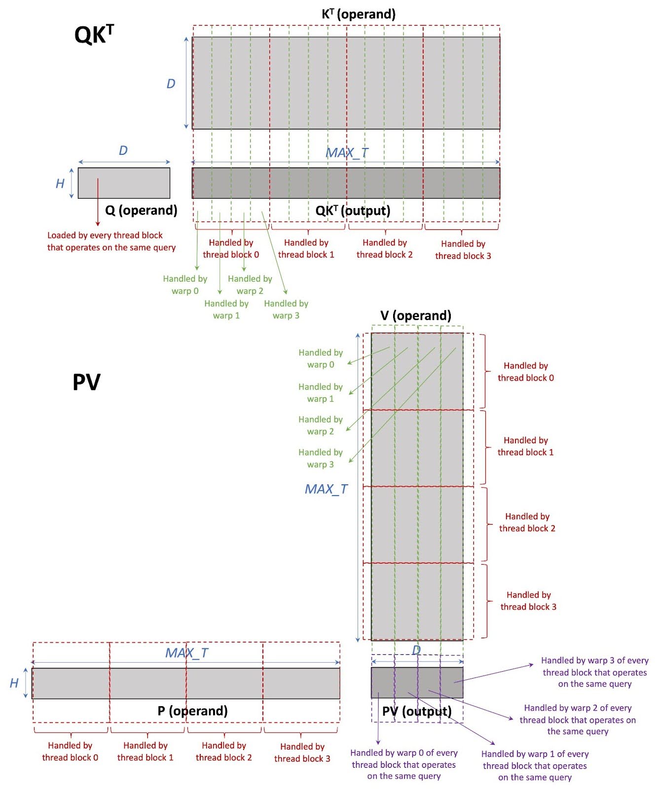
Figure 4 CU work partitioning
Optimizing CUDA with Tensor Cores Kernel of INT4 GQA
In this note, we discuss the optimizations that we have applied to the CUDA with tensor cores implementation of INT4 GQA (CU). The ideal goal is to improve the INT4 GQA performance by 4 times based on the CI analysis in the previous section. Note that the query size is negligible compared to the KV cache size when the context length is long.
In our analysis, we used the NVIDIA Nsight Compute (NCU) as the main profiler. Our general bottleneck elimination approach is to minimize the stall cycles. We applied 10 optimizations to INT4 GQA, three of which are specific for NVIDIA A100/H100 GPUs. These optimizations are well known CUDA optimization techniques which can be generalized to many applications.
It is worth noting that the reason that we choose to optimize the CUDA implementation rather than the Flash-Decoding implementation (FD) (which is Triton based) is because with CUDA, we have a better control of how the low-level instructions are being generated. Many optimization techniques that we apply such as, operating on tensor core fragments directly (Optimizations 7-9), cannot be done through Triton since it does not expose low-level details to developers. However, these optimizations can be integrated into the compiler-based solution to make the optimizations available to broader operators, which is indeed a part of our future plan.
Optimization 1: Unroll K Loads
Problem Analysis:
The NCU profile shows that during K loading, there are only 2 global loads followed by memory stalls at dequantize_permuted_int4. The memory stalls are the long scoreboard stalls which indicates the waits for global memory access. This suggests that the kernel does not issue sufficient memory loads
to hide the global load latency. The kernel issues data loading, and then waits to consume the data immediately causing the global load latency to be exposed. The stalls are shown in Figure 5.
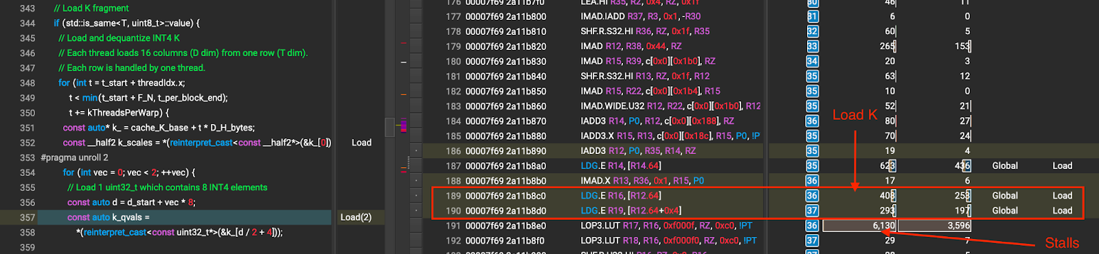
Figure 5 K loading before unrolling (the numbers that the arrows point to are stall cycles caused by global memory wait)
Solution:
In the baseline implementation, we use uint32_t to load 8 INT4 K values in a single load and we perform 2 uint32_t loads in each iteration, which is 16 INT4 K values. To allow for a better global load latency hiding, we issue 8 uint32_t loads instead of two before consuming the K values in dequantize_permuted_int4. This allows the compiler to unroll the loads as well as reorder the instructions to hide the global load latency better. Figure 6 shows the NCU profile of K loading after unrolling. Comparing Figure 5 and Figure 6, we effectively reduce the stall cycles by unrolling the K loads.
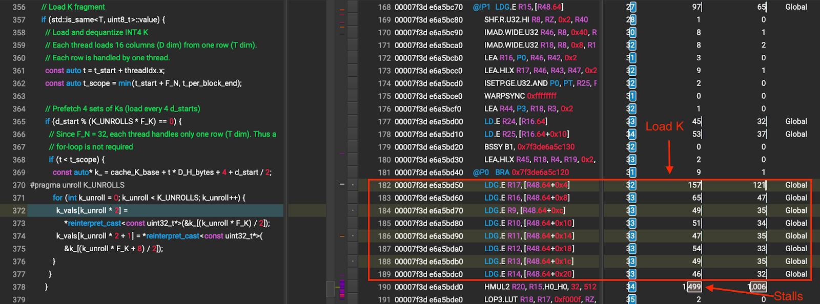
Figure 6 K loading after unrolling (the numbers that the arrows point to are stall cycles caused by global memory wait)
Results:
Table 3 Performance of Optimization 1 for INT4 GQA (row-wise quantization)
| Batch size | Time (us) | Bandwidth (GB/s) | Speed up | |||||
| FD | CU | FD | CU | vs FD | vs CU baseline | |||
| Baseline | Opt 1 | Baseline | Opt 1 | |||||
| 32 | 137 | 143 | 134 | 262 | 250 | 267 | 1.02 | 1.07 |
| 64 | 234 | 257 | 237 | 305 | 278 | 302 | 0.99 | 1.09 |
| 128 | 432 | 455 | 422 | 331 | 314 | 339 | 1.02 | 1.08 |
| 256 | 815 | 866 | 806 | 351 | 331 | 355 | 1.01 | 1.07 |
| 512 | 1581 | 1659 | 1550 | 362 | 345 | 369 | 1.02 | 1.07 |
Optimization 2: Improve P Type Casting (FP32->BF16)
Problem Analysis:
Since the product of softmax(bmm(Q, KT) / sqrt(D)) is FP32 (denoted as P in Figure 3), the kernel has to convert P from FP32 to BF16 before feeding it to the next bmm computation. The kernel performs the FP32 to BF16 conversion of P by copying the FP32 data from one location in shared memory to another location in shared memory. This causes stalls during the shared memory access (shown in Figure 7) which might be caused by (1) the shared memory indirection; and (2) the shared memory bank conflict since each thread accesses an 16-bit element (because of this, two threads can access the same memory bank simultaneously).
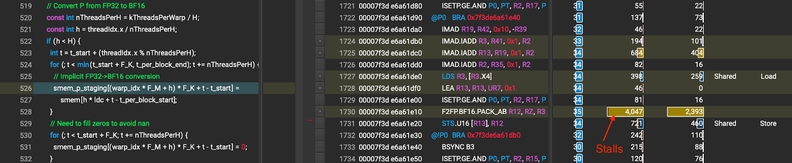
Figure 7 P type casting before Optimization 2 (the number that the arrow points to is stall cycles caused by shared memory wait)
Solution:
We use all threads in the thread block to do in-place type conversion. Each thread operates on two consecutive elements in order to avoid the shared memory bank conflict when storing BF16. All threads work on the same head (h) at the same time to guarantee correctness of the conversion. The in-place conversion steps are as follows:
- Each thread loads 2 FP32 token elements from the same head from the shared memory into registers
- Call
__syncthreads()to make sure that every thread finishes reading the data - Each thread converts its data to 2 BF16 token elements and then stores the results to the same shared memory
Some optimizations that we apply to the implementation:
- Use vector types (especially
nv_bfloat2) - Unroll data loading/storing, i.e., performing multiple loads before calling
__syncthreads()and performing multiple stores after__syncthreads()
After this optimization, long stalls are not observed during P type casting as shown in Figure 8.
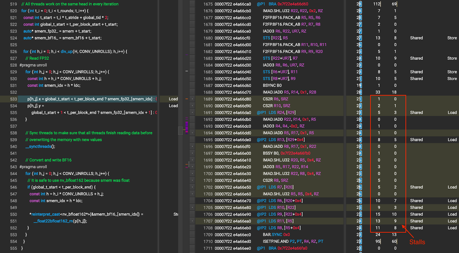
Figure 8 P type casting after Optimization 2 (the numbers that the arrow points to are stall cycles caused by shared memory wait)
Culprits:
Since we unroll data loading/storing by using registers as an intermediate storage, the number of registers per thread increases resulting in reduced occupancy.
Results:
Table 4 Performance of Optimization 2 for INT4 GQA (row-wise quantization)
| Batch size | Time (us) | Bandwidth (GB/s) | Speed up | |||||
| FD | CU | FD | CU | vs FD | vs CU baseline | |||
| Baseline | Opt 2 | Baseline | Opt 2 | |||||
| 32 | 137 | 143 | 126 | 262 | 250 | 285 | 1.09 | 1.14 |
| 64 | 234 | 257 | 221 | 305 | 278 | 324 | 1.06 | 1.16 |
| 128 | 432 | 455 | 395 | 331 | 314 | 362 | 1.09 | 1.15 |
| 256 | 815 | 866 | 749 | 351 | 331 | 382 | 1.09 | 1.16 |
| 512 | 1581 | 1659 | 1435 | 362 | 345 | 399 | 1.10 | 1.16 |
Optimization 3: Remove Local Memory Usage for max QKT computation
Problem Analysis:
During the softmax computation, the kernel has to compute max QKT for each head. It uses a temporary “thread-local” storage for storing per-thread max QKT results (one float value for each head). Depending on the compiler, the thread-local storage can be allocated on registers (on chip) or the local memory (off chip == global memory). Unfortunately, in the baseline, the thread-local storage resides in the local memory which is much slower than the registers (shown in Figure 9). We suspect that this is because the compiler cannot determine the indices of thread-local storage at compile time (since the number of heads (H) in the kernel is a runtime variable). Accessing local memory as if accessing registers can hurt the performance of the kernel.
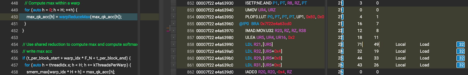
Figure 9 Local memory access during max QKT computation
Solution:
We realize that we do not need H (number of heads) floats as temporary storage per thread since each thread can compute max QKT for only one head instead of all the heads. Thus, we only need one float per thread, which can be easily stored in a register. To accumulate the max results among warps, we use shared memory. This optimization eliminates the local memory usage during max QKT computation.
Results:
Table 5 Performance of Optimization 3 for INT4 GQA (row-wise quantization)
| Batch size | Time (us) | Bandwidth (GB/s) | Speed up | |||||
| FD | CU | FD | CU | vs FD | vs CU baseline | |||
| Baseline | Opt 3 | Baseline | Opt 3 | |||||
| 32 | 137 | 143 | 119 | 262 | 250 | 300 | 1.14 | 1.20 |
| 64 | 234 | 257 | 206 | 305 | 278 | 348 | 1.14 | 1.25 |
| 128 | 432 | 455 | 368 | 331 | 314 | 389 | 1.17 | 1.24 |
| 256 | 815 | 866 | 696 | 351 | 331 | 411 | 1.17 | 1.24 |
| 512 | 1581 | 1659 | 1338 | 362 | 345 | 428 | 1.18 | 1.24 |
Optimization 4: Remove local memory usage for row sum
Problem Analysis:
Similar to Optimization 3, the local memory usage problem is also observed during the row sum computation in the softmax computation. Since local memory is off chip, accessing it as if accessing registers can hurt the performance of the kernel.
Solution:
We apply the same solution as the max QKT computation for the row sum computation. That is to have each thread compute a row sum of only one head, which requires only one float per thread. This eliminates the need for local memory.
Results:
Table 6 Performance of Optimization 4 for INT4 GQA (row-wise quantization)
| Batch size | Time (us) | Bandwidth (GB/s) | Speed up | |||||
| FD | CU | FD | CU | vs FD | vs CU baseline | |||
| Baseline | Opt 4 | Baseline | Opt 4 | |||||
| 32 | 137 | 143 | 118 | 262 | 250 | 302 | 1.15 | 1.21 |
| 64 | 234 | 257 | 204 | 305 | 278 | 351 | 1.15 | 1.26 |
| 128 | 432 | 455 | 364 | 331 | 314 | 393 | 1.19 | 1.25 |
| 256 | 815 | 866 | 688 | 351 | 331 | 416 | 1.18 | 1.26 |
| 512 | 1581 | 1659 | 1328 | 362 | 345 | 431 | 1.19 | 1.25 |
Optimization 5: Add prefetch for V load
Problem Analysis:
The same issue as K loading is observed when loading V. That is, the kernel issues data loading, and then waits to consume the data immediately causing the global load latency to be exposed. However, when using the unrolling technique mentioned above, the compiler allocates the temporary buffer on local memory instead of registers causing a large slow down.
Solution:
We adopt the data prefetching technique for V loading. We load the next iteration V values immediately after the current iteration values are consumed. This allows the data loading to be overlapped with the PK computation resulting in better kernel performance.
Results:
Table 7 Performance of Optimization 5 for INT4 GQA (row-wise quantization)
| Batch size | Time (us) | Bandwidth (GB/s) | Speed up | |||||
| FD | CU | FD | CU | vs FD | vs CU baseline | |||
| Baseline | Opt 5 | Baseline | Opt 5 | |||||
| 32 | 137 | 143 | 109 | 262 | 250 | 327 | 1.25 | 1.31 |
| 64 | 234 | 257 | 194 | 305 | 278 | 370 | 1.21 | 1.33 |
| 128 | 432 | 455 | 345 | 331 | 314 | 414 | 1.25 | 1.32 |
| 256 | 815 | 866 | 649 | 351 | 331 | 441 | 1.26 | 1.33 |
| 512 | 1581 | 1659 | 1244 | 362 | 345 | 460 | 1.27 | 1.33 |
Optimization 6: Add Group-Wise INT4 (Groups = 4) with Vector Load
Problem Analysis:
Prior to this optimization, CU only supported row-wise INT4 quantization. That is, every column in each row shares the same scales. The scales of each row are stored in the first 4 bytes of each row as shown in Figure 10. In the kernel, each thread loads only one row at a time. Since each row contains 68 bytes (4 bytes for scales and 64 bytes for data), it cannot guarantee that every row aligns with a size of any vector type. Thus, vector loads cannot be used for loading the KV cache.
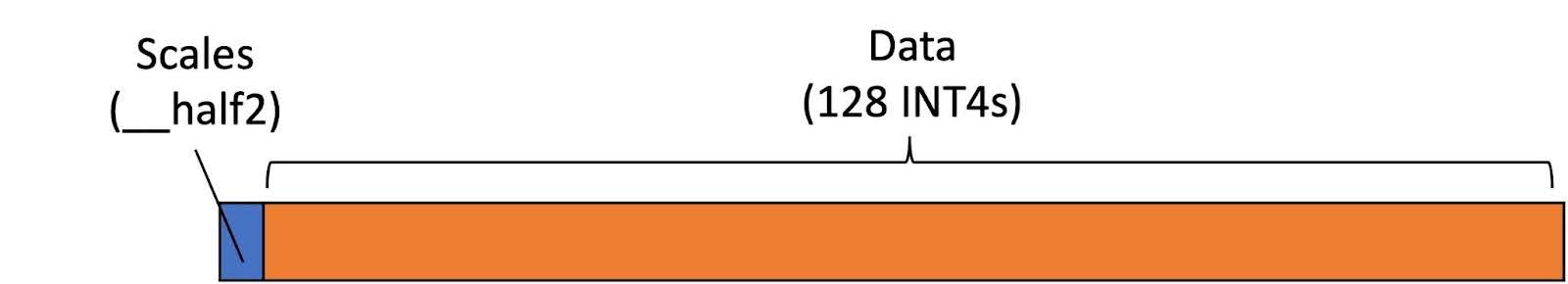
Figure 10 The layout of each row of INT4 KV cache with row-wise quantization
Solution:
We have implemented support for group-wise INT4 quantization with num groups = 4. In this case, columns in each row in the KV cache tensor are divided into 4 equal groups. Columns within the same group share the same scales for quantization/dequantization. The data layout for INT4 KV cache is shown in Figure 11. The scales for all groups are serialized and stored at the beginning of each row. The INT4 data is also serialized and laid out next to the scales.
Because the number of bytes in each row now becomes 80 bytes, we can use a vector type, i.e., uint2 in our case, to load data. (We do not use uint4 since each thread loads only 16 INT4s at a time due to the tensor core fragment size.) Vector load is generally better than scalar load since it does not cause extra byte loads.
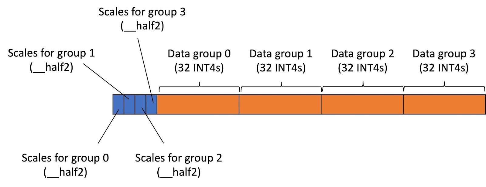
Figure 11 The layout of each row of INT4 KV cache with row-wise quantization
Results:
Table 8 Performance of Optimization 6 for INT4 GQA (row-wise quantization)
| Batch size | Time (us) | Bandwidth (GB/s) | Speed up | |||||
| FD | CU | FD | CU | vs FD | vs CU baseline | |||
| Baseline | Opt 6 | Baseline | Opt 6 | |||||
| 32 | 137 | 143 | 111 | 262 | 250 | 322 | 1.23 | 1.29 |
| 64 | 234 | 257 | 192 | 305 | 278 | 372 | 1.22 | 1.34 |
| 128 | 432 | 455 | 346 | 331 | 314 | 414 | 1.25 | 1.32 |
| 256 | 815 | 866 | 642 | 351 | 331 | 446 | 1.27 | 1.35 |
| 512 | 1581 | 1659 | 1244 | 362 | 345 | 460 | 1.27 | 1.33 |
Table 9 Performance of Optimization 6 for INT4 GQA (group-wise quantization with num groups = 4)
| Batch size | Time (us) | Bandwidth (GB/s) | Speed up | ||
| FD | CUDA_WMMA | FD | CUDA_WMMA | vs FD | |
| Opt 6 | Opt 6 | ||||
| 32 | 129 | 116 | 325 | 364 | 1.31 |
| 64 | 219 | 195 | 385 | 431 | 1.36 |
| 128 | 392 | 347 | 429 | 484 | 1.39 |
| 256 | 719 | 638 | 468 | 527 | 1.41 |
| 512 | 1375 | 1225 | 489 | 550 | 1.43 |
Optimization 7: Compute max QKT From WMMA Fragment Directly (A100/H100 specific)
Problem Analysis:
We observe large stalls due to shared memory accessing during the max QKT computation (showing as large short scoreboard stalls) as shown in Figure 12.
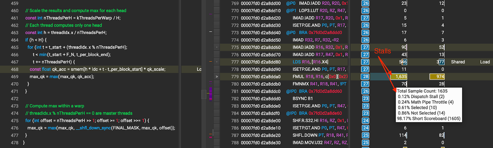
Figure 12 Stalls due to shared memory access during max QKT computation (the number that the arrow points to is stall cycles caused by shared memory wait)
Solution:
We bypass shared memory when computing max QKT by computing it from the WMMA fragment (i.e., the tensor core fragment) directly. The layout of the WMMA fragment is specific to the GPU architecture. In this optimization, we only enabled this optimization for the NVIDIA A100/H100 GPUs. Other GPUs will still use shared memory for the max QKT computation. By bypassing shared memory, we effectively eliminate the stalls caused by shared memory access. The tensor core layout of the C fragment which is used for storing the QKT results is shown in Figure 13.
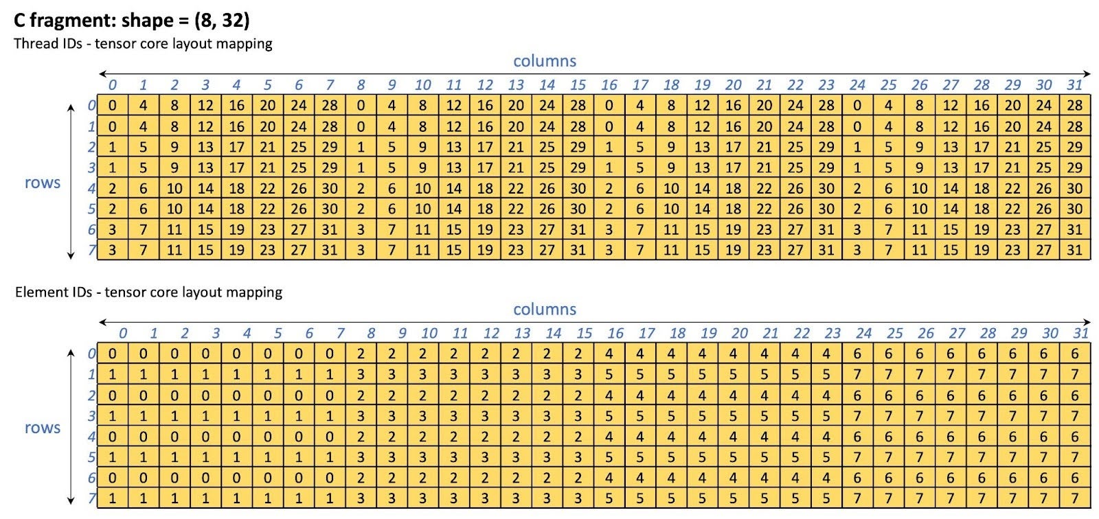
Figure 13 C fragment (QKT storage) tensor core layout on A100/H100
Table 10 Performance of Optimization 7 for INT4 GQA (row-wise quantization)
| Batch size | Time (us) | Bandwidth (GB/s) | Speed up | |||||
| FD | CU | FD | CU | vs FD | vs CU baseline | |||
| Baseline | Opt 7 | Baseline | Opt 7 | |||||
| 32 | 137 | 143 | 107 | 262 | 250 | 333 | 1.27 | 1.33 |
| 64 | 234 | 257 | 183 | 305 | 278 | 391 | 1.28 | 1.40 |
| 128 | 432 | 455 | 333 | 331 | 314 | 430 | 1.30 | 1.37 |
| 256 | 815 | 866 | 620 | 351 | 331 | 461 | 1.31 | 1.40 |
| 512 | 1581 | 1659 | 1206 | 362 | 345 | 475 | 1.31 | 1.38 |
Table 11 Performance of Optimization 7 for INT4 GQA (group-wise quantization with num groups = 4)
| Batch size | Time (us) | Bandwidth (GB/s) | Speed up | |||||
| FD | CUDA_WMMA | FD | CUDA_WMMA | vs FD | vs CUDA_WMMA Opt 6 | |||
| Opt 6 | Opt 7 | Opt 6 | Opt 7 | |||||
| 32 | 129 | 116 | 111 | 325 | 364 | 380 | 1.17 | 1.04 |
| 64 | 219 | 195 | 187 | 385 | 431 | 449 | 1.17 | 1.04 |
| 128 | 392 | 347 | 333 | 429 | 484 | 506 | 1.18 | 1.04 |
| 256 | 719 | 638 | 615 | 468 | 527 | 547 | 1.17 | 1.04 |
| 512 | 1375 | 1225 | 1184 | 489 | 550 | 569 | 1.16 | 1.03 |
Optimization 8: Write FP32->BF16 Results to P Fragment Directly (A100/H100 specific)
Problem Analysis:
During the FP32-BF16 conversion for the P fragment, the kernel loads the FP32 data from shared memory, does the conversion and then stores the BF16 data back to shared memory. Moreover, the conversion requires many thread block synchronizations (__syncthreads()).
Solution:
Due to the data partitioning design of the kernel, each warp performs only one pass through the P fragment. Thus, we do not have to write the conversion results back to the shared memory for future usage. To avoid writing the BF16 data to the shared memory and thread block synchronizations, we have each warp load the FP32 data of the P WMMA fragment from the shared memory, do the conversion and then write the BF16 data directly to the P fragment.
Note that this optimization is applied to only the NVIDIA A100 and H100 GPUs because the WMMA fragment layout is architecture dependent. For non-A100/H100 GPUs, the kernel will fallback to the original path.
The P fragment tensor core layout is shown in Figure 14. Note that this layout is specific to the NVIDIA A100/H100 GPU.
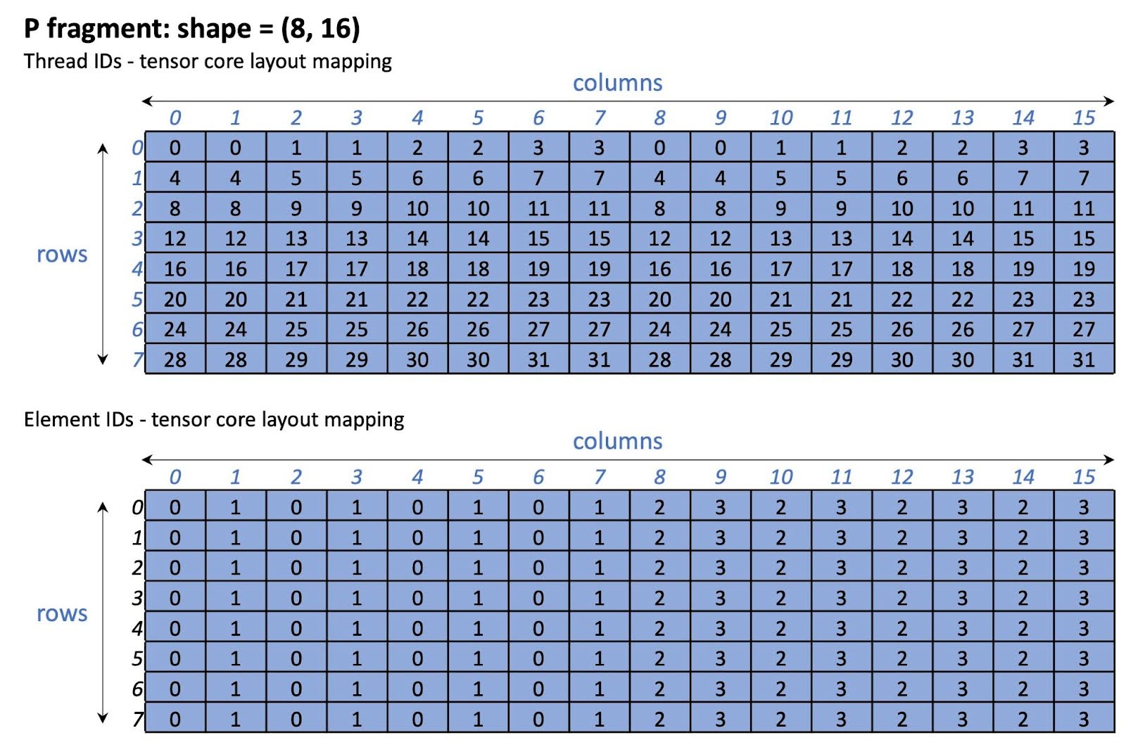
Figure 14 P fragment tensor core layout on A100/H100
Table 12 Performance of Optimization 8 for INT4 GQA (row-wise quantization)
| Batch size | Time (us) | Bandwidth (GB/s) | Speed up | |||||
| FD | CU | FD | CU | vs FD | vs CU baseline | |||
| Baseline | Opt 8 | Baseline | Opt 8 | |||||
| 32 | 137 | 143 | 101 | 262 | 250 | 353 | 1.35 | 1.41 |
| 64 | 234 | 257 | 174 | 305 | 278 | 410 | 1.34 | 1.47 |
| 128 | 432 | 455 | 317 | 331 | 314 | 451 | 1.36 | 1.43 |
| 256 | 815 | 866 | 590 | 351 | 331 | 485 | 1.38 | 1.47 |
| 512 | 1581 | 1659 | 1143 | 362 | 345 | 501 | 1.38 | 1.45 |
Table 13 Performance of Optimization 8 for INT4 GQA (group-wise quantization with num groups = 4)
| Batch size | Time (us) | Bandwidth (GB/s) | Speed up | |||||
| FD | CUDA_WMMA | FD | CUDA_WMMA | vs FD | vs CUDA_WMMA Opt 6 | |||
| Opt 6 | Opt 8 | Opt 6 | Opt 8 | |||||
| 32 | 129 | 116 | 106 | 325 | 364 | 396 | 1.22 | 1.09 |
| 64 | 219 | 195 | 180 | 385 | 431 | 467 | 1.21 | 1.08 |
| 128 | 392 | 347 | 319 | 429 | 484 | 528 | 1.23 | 1.09 |
| 256 | 719 | 638 | 596 | 468 | 527 | 565 | 1.21 | 1.07 |
| 512 | 1375 | 1225 | 1138 | 489 | 550 | 591 | 1.21 | 1.08 |
Optimization 9: Swizzle P Shared Memory Layouts (A100/H100 specific)
Problem Analysis:
We observe large shared memory bank conflicts during P loading. The amount of bank conflict depends on the memory access stride. For instance, for split-Ks = 32 and max seq length = 8192, we observed that only 4 out of 32 banks are being accessed in parallel (memory access stride = 256). From Figure 14, when all threads access element 0, threads that have the same threadIdx.x % 4 access the same bank.
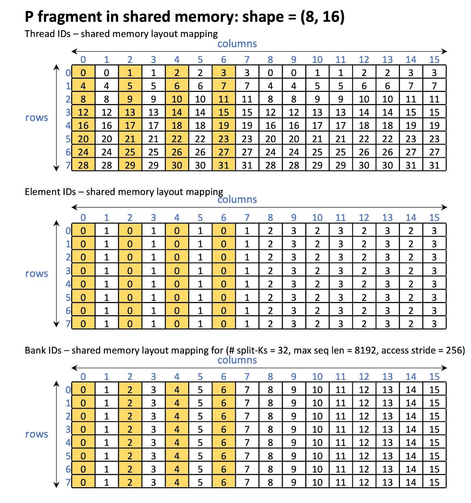
Figure 15 P fragment in shared memory before swizzling
Solution:
We shuffle the layout of P load/store in the shared memory in such a way that avoids bank conflicts. In other words, we store the QKT results (C fragment) and load them (P fragment) using the swizzled layout. Moreover, instead of using the original memory access stride which is dependent on the number of tokens per thread block, we use the fragment’s column size as the stride which is constant. Thus, the load and store of the P fragment is always contiguous.
The new layouts for the C and P fragments are shown in Figure 16. With the new layout, it is guaranteed that 16 banks are being accessed in parallel as shown in Figure 17.
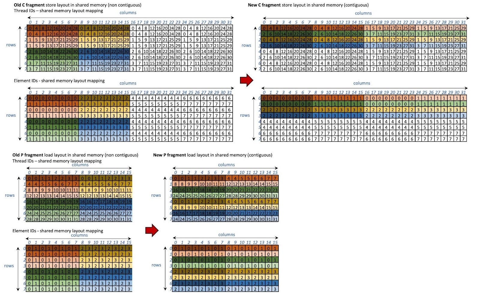
Figure 16 The swizzled layouts of C and P fragments
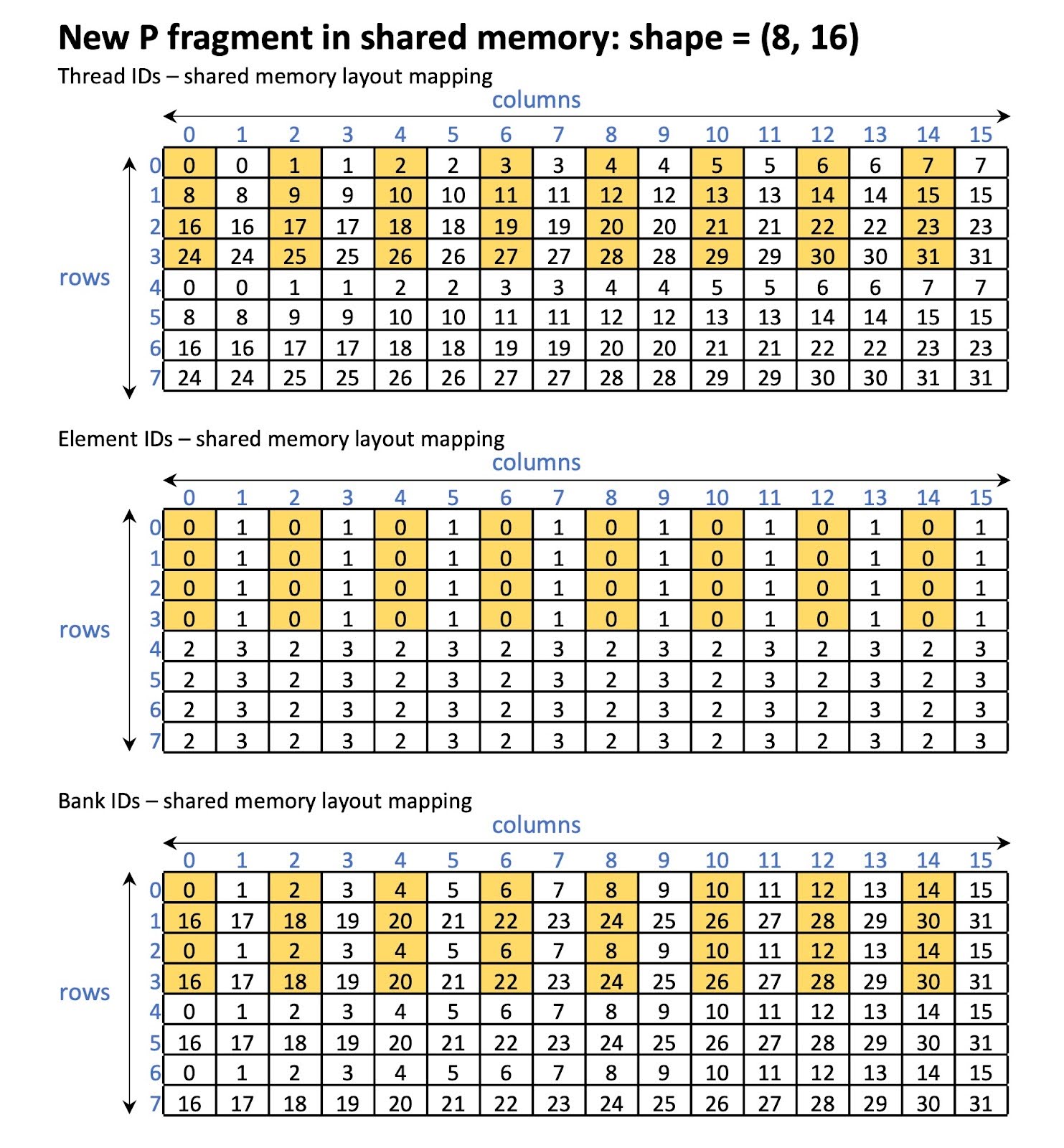
Figure 17 P fragment in shared memory after swizzling
Table 14 Performance of Optimization 9 for INT4 GQA (row-wise quantization)
| Batch size | Time (us) | Bandwidth (GB/s) | Speed up | |||||
| FD | CU | FD | CU | vs FD | vs CU baseline | |||
| Baseline | Opt 9 | Baseline | Opt 9 | |||||
| 32 | 137 | 143 | 98 | 262 | 250 | 365 | 1.39 | 1.46 |
| 64 | 234 | 257 | 167 | 305 | 278 | 429 | 1.41 | 1.54 |
| 128 | 432 | 455 | 299 | 331 | 314 | 479 | 1.45 | 1.52 |
| 256 | 815 | 866 | 549 | 351 | 331 | 521 | 1.48 | 1.58 |
| 512 | 1581 | 1659 | 1060 | 362 | 345 | 540 | 1.49 | 1.56 |
Table 15 Performance of Optimization 9 for INT4 GQA (group-wise quantization with num groups = 4)
| Batch size | Time (us) | Bandwidth (GB/s) | Speed up | |||||
| FD | CUDA_WMMA | FD | CUDA_WMMA | vs FD | vs CUDA_WMMA Opt 6 | |||
| Opt 6 | Opt 9 | Opt 6 | Opt 9 | |||||
| 32 | 129 | 116 | 105 | 325 | 364 | 400 | 1.23 | 1.10 |
| 64 | 219 | 195 | 174 | 385 | 431 | 484 | 1.26 | 1.12 |
| 128 | 392 | 347 | 302 | 429 | 484 | 558 | 1.30 | 1.15 |
| 256 | 719 | 638 | 560 | 468 | 527 | 601 | 1.28 | 1.14 |
| 512 | 1375 | 1225 | 1065 | 489 | 550 | 632 | 1.29 | 1.15 |
Optimization 10: Pad Shared Memory for INT4 Dequantization
Problem Analysis:
Once the kernel reads the INT4 K or V cache from global memory, it performs dequantization and stores the results (BF16) in the shared memory. Then, the BF16 data is loaded to the WMMA fragment from shared memory (via the WMMA interface). We observed a large number of bank conflicts for both K and V accesses. For instance, for K stores, only 4 out of 32 banks are being accessed in parallel. For K loads, 16 banks are being accessed in parallel. The same also occurs for V stores and loads. See the figures in the solution section.
Solution:
We pad the shared memory to reduce the bank conflict. Specifically, we pad each row by 2. That is, the row stride of K becomes F_K + 2 and the row stride of V becomes F_N + 2 (F_K and F_N are the fixed widths of the K and V WMMA fragments, respectively). With this optimization, we are able to reduce the bank conflict by 1.8x as shown in Figure 18.
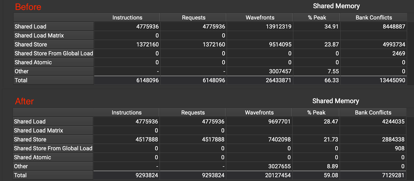
Figure 18 Bank conflicts before and after Optimization 10
After Optimization 10, for K stores, 32 banks are being accessed in parallel (shown in Figure 19), while for K loads, 29 banks are accessed in parallel (shown in Figure 20).
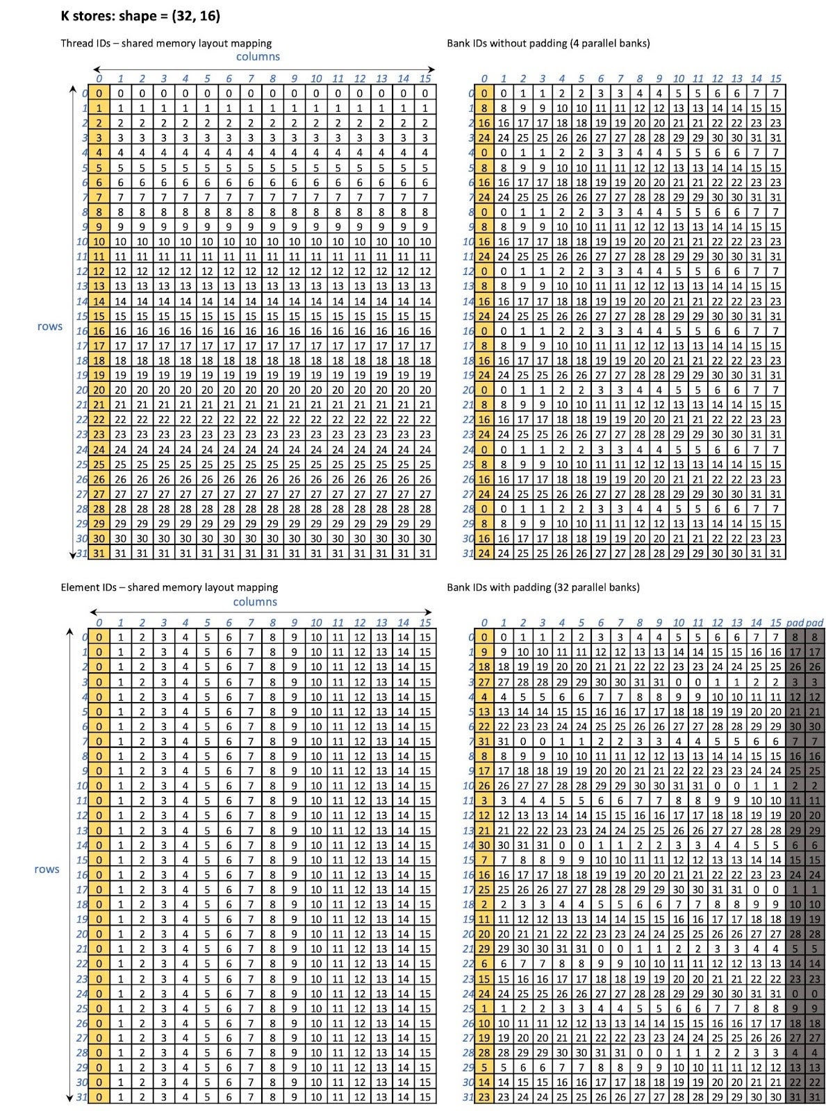
Figure 19 K fragment store shared memory layout without and with padding
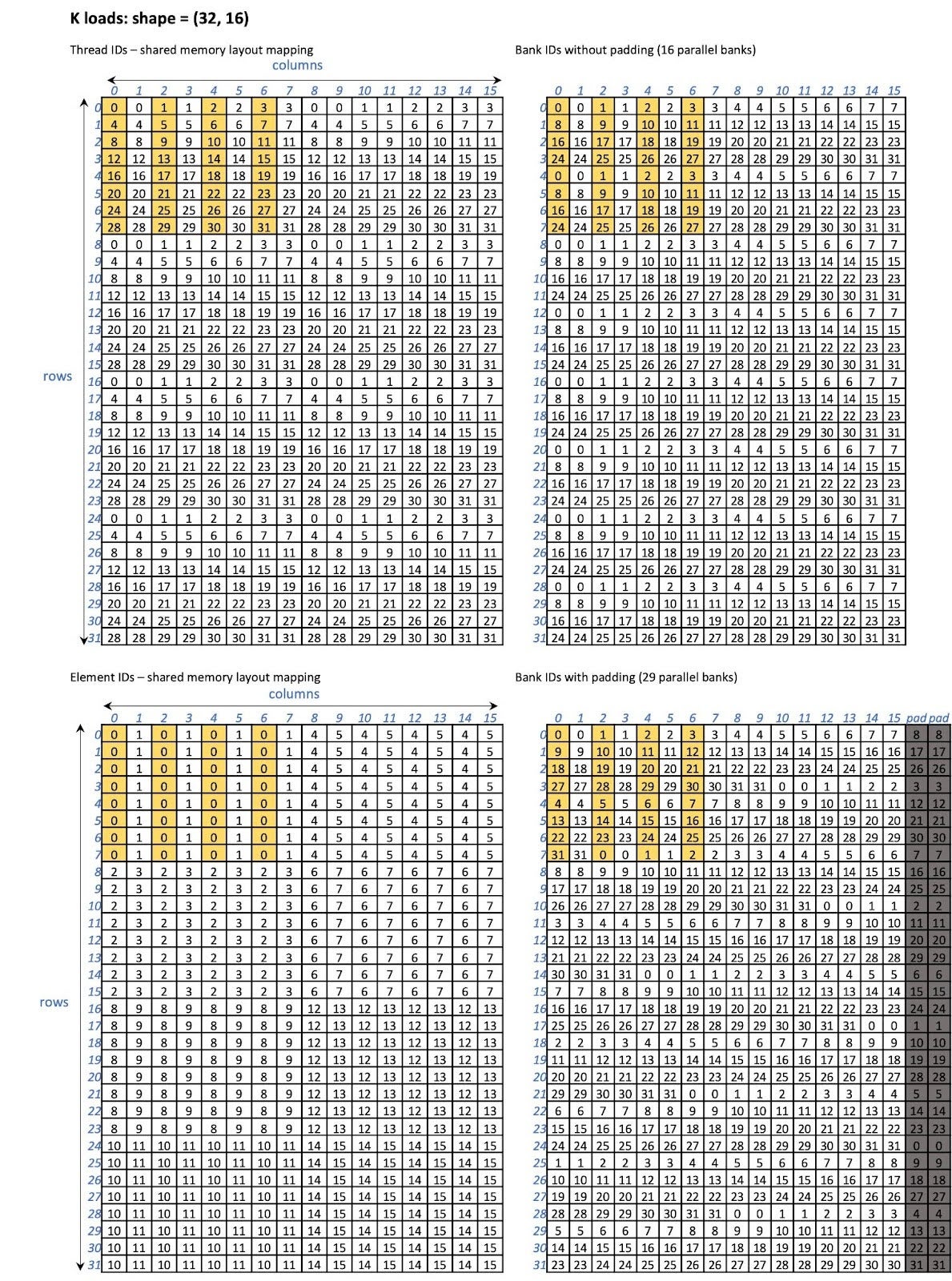
Figure 20 K fragment load shared memory layout without and with padding
Table 16 Performance of Optimization 10 for INT4 GQA (row-wise quantization)
| Batch size | Time (us) | Bandwidth (GB/s) | Speed up | |||||
| FD | CU | FD | CU | vs FD | vs CU baseline | |||
| Baseline | Opt 10 | Baseline | Opt 10 | |||||
| 32 | 137 | 143 | 94 | 262 | 250 | 380 | 1.45 | 1.52 |
| 64 | 234 | 257 | 151 | 305 | 278 | 475 | 1.55 | 1.71 |
| 128 | 432 | 455 | 266 | 331 | 314 | 538 | 1.63 | 1.71 |
| 256 | 815 | 866 | 489 | 351 | 331 | 586 | 1.67 | 1.77 |
| 512 | 1581 | 1659 | 930 | 362 | 345 | 616 | 1.70 | 1.79 |
Table 17 Performance of Optimization 10 for INT4 GQA (group-wise quantization with num groups = 4)
| Batch size | Time (us) | Bandwidth (GB/s) | Speed up | |||||
| FD | CUDA_WMMA | FD | CUDA_WMMA | vs FD | vs CUDA_WMMA Opt 6 | |||
| Opt 6 | Opt 10 | Opt 6 | Opt 10 | |||||
| 32 | 129 | 116 | 99 | 325 | 364 | 425 | 1.31 | 1.17 |
| 64 | 219 | 195 | 161 | 385 | 431 | 523 | 1.36 | 1.21 |
| 128 | 392 | 347 | 282 | 429 | 484 | 598 | 1.39 | 1.23 |
| 256 | 719 | 638 | 509 | 468 | 527 | 662 | 1.41 | 1.25 |
| 512 | 1375 | 1225 | 965 | 489 | 550 | 698 | 1.43 | 1.27 |
Performance Evaluation
Microbenchmark results
We also evaluated BF16 GQA performance using our optimized kernel (as shown in Table 19). CU still performs generally worse than FD and FA for BF16. This is expected since our optimizations are INT4 focused.
While INT4 GQA is still not as efficient as BF16 GQA (see the achieved bandwidths), it is important to note that when comparing FD BF16 GQA performance against CU INT4 GQA performance, we can see that the latency of INT4 is smaller than that of BF16.
Table 19 Performance of BF16 GQA and INT GQA after CU optimizations
On A100
| Time (us) | BF16 GQA | INT4 GQA | ||||||
| Batch size | FD | FA | CU before | CU after | FD | FA | CU before | CU after |
| 32 | 139 | 133 | 183 | 163 | 137 | – | 143 | 94 |
| 64 | 245 | 229 | 335 | 276 | 234 | – | 257 | 151 |
| 128 | 433 | 555 | 596 | 517 | 432 | – | 455 | 266 |
| 256 | 826 | 977 | 1127 | 999 | 815 | – | 866 | 489 |
| 512 | 1607 | 1670 | 2194 | 1879 | 1581 | – | 1659 | 930 |
| Effective Bandwidth (GB/s) | BF16 GQA | INT4 GQA | ||||||
| Batch size | FD | FA | CU before | CU after | FD | FA | CU before | CU after |
| 32 | 965 | 1012 | 736 | 824 | 262 | – | 250 | 380 |
| 64 | 1097 | 1175 | 802 | 972 | 305 | – | 278 | 475 |
| 128 | 1240 | 968 | 901 | 1039 | 331 | – | 314 | 538 |
| 256 | 1301 | 1100 | 954 | 1075 | 351 | – | 331 | 586 |
| 512 | 1338 | 1287 | 980 | 1144 | 362 | – | 345 | 616 |
On H100
| Time (us) | BF16 GQA | INT4 GQA | ||||||
| Batch size | FD | FA | CU before | CU after | FD | FA | CU before | CU after |
| 32 | 91 | 90 | 114 | 100 | 70 | – | 96 | 64 |
| 64 | 148 | 146 | 200 | 183 | 113 | – | 162 | 101 |
| 128 | 271 | 298 | 361 | 308 | 205 | – | 294 | 170 |
| 256 | 515 | 499 | 658 | 556 | 389 | – | 558 | 306 |
| 512 | 1000 | 1011 | 1260 | 1066 | 756 | – | 1066 | 575 |
| Effective Bandwidth (GB/s) | BF16 GQA | INT4 GQA | ||||||
| Batch size | FD | FA | CU before | CU after | FD | FA | CU before | CU after |
| 32 | 1481 | 1496 | 1178 | 1341 | 511 | – | 371 | 560 |
| 64 | 1815 | 1840 | 1345 | 1470 | 631 | – | 443 | 710 |
| 128 | 1982 | 1802 | 1487 | 1743 | 699 | – | 487 | 844 |
| 256 | 2087 | 2156 | 1634 | 1934 | 736 | – | 513 | 935 |
| 512 | 2150 | 2127 | 1706 | 2015 | 757 | – | 537 | 996 |
E2E results
We evaluated our optimized INT4 GQA kernel in Llama 2 70B on 8 H100 GPUs. We ran the model end-to-end, but only reported the decode latency. We use FP8 FFN (feed forward network) to emphasize the attention performance in the decoding phase. We vary the batch size from 1 to 256 and the context length from 2,048 (2K) to 16,384 (16K). The E2E performance results are shown in the figure below.
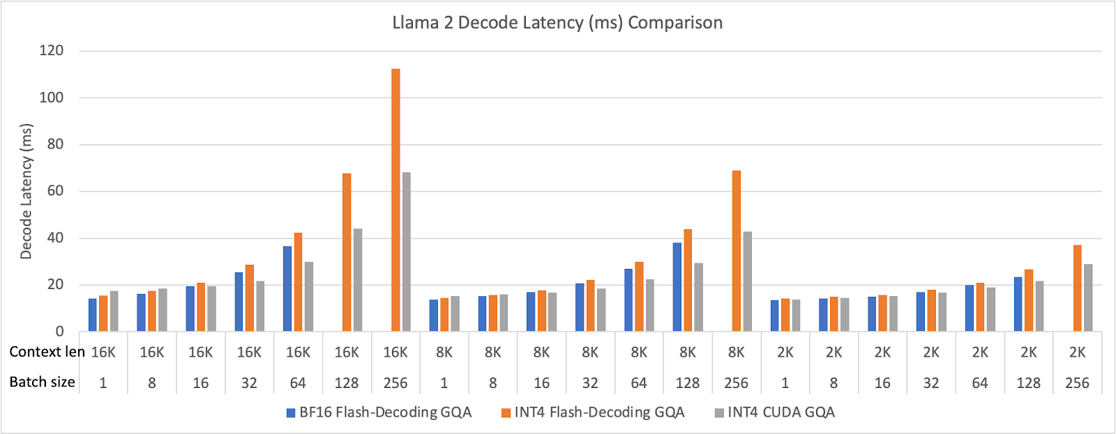
Figure 21 Meta Llama 2 decode latency (ms) comparison (BF16 GQA runs out of memory in large batch size configurations)
Code
If you are interested, please checkout our code here. If you have any questions, please feel free to open an issue on GitHub, and we will be happy to help. Your contributions are welcome!