In this blogpost we describe the recently proposed Stochastic Weight Averaging (SWA) technique [1, 2], and its new implementation in torchcontrib. SWA is a simple procedure that improves generalization in deep learning over Stochastic Gradient Descent (SGD) at no additional cost, and can be used as a drop-in replacement for any other optimizer in PyTorch. SWA has a wide range of applications and features:
- SWA has been shown to significantly improve generalization in computer vision tasks, including VGG, ResNets, Wide ResNets and DenseNets on ImageNet and CIFAR benchmarks [1, 2].
- SWA provides state-of-the-art performance on key benchmarks in semi-supervised learning and domain adaptation [2].
- SWA is shown to improve the stability of training as well as the final average rewards of policy-gradient methods in deep reinforcement learning [3].
- An extension of SWA can obtain efficient Bayesian model averaging, as well as high quality uncertainty estimates and calibration in deep learning [4].
- SWA for low precision training, SWALP, can match the performance of full-precision SGD even with all numbers quantized down to 8 bits, including gradient accumulators [5].
In short, SWA performs an equal average of the weights traversed by SGD with a modified learning rate schedule (see the left panel of Figure 1.). SWA solutions end up in the center of a wide flat region of loss, while SGD tends to converge to the boundary of the low-loss region, making it susceptible to the shift between train and test error surfaces (see the middle and right panels of Figure 1).
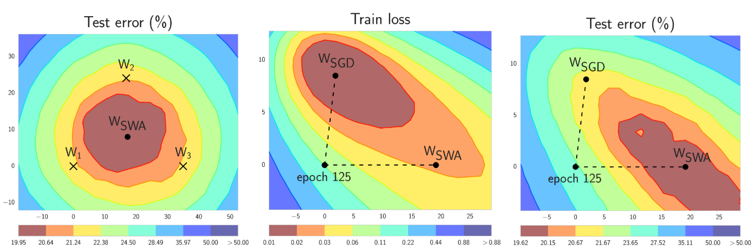
Figure 1. Illustrations of SWA and SGD with a Preactivation ResNet-164 on CIFAR-100 [1]. Left: test error surface for three FGE samples and the corresponding SWA solution (averaging in weight space). Middle and Right: test error and train loss surfaces showing the weights proposed by SGD (at convergence) and SWA, starting from the same initialization of SGD after 125 training epochs. Please see [1] for details on how these figures were constructed.
With our new implementation in torchcontrib using SWA is as easy as using any other optimizer in PyTorch:
from torchcontrib.optim import SWA

...
...

# training loop
base_opt = torch.optim.SGD(model.parameters(), lr=0.1)
opt = torchcontrib.optim.SWA(base_opt, swa_start=10, swa_freq=5, swa_lr=0.05)
for _ in range(100):
     opt.zero_grad()
     loss_fn(model(input), target).backward()
     opt.step()
opt.swap_swa_sgd()
You can wrap any optimizer from torch.optim using the SWA class, and then train your model as usual. When training is complete you simply call swap_swa_sgd() to set the weights of your model to their SWA averages. Below we explain the SWA procedure and the parameters of the SWA class in detail. We emphasize that SWA can be combined with any optimization procedure, such as Adam, in the same way that it can be combined with SGD.
Is this just Averaged SGD?
At a high level, averaging SGD iterates dates back several decades in convex optimization [6, 7], where it is sometimes referred to as Polyak-Ruppert averaging, or averaged SGD. But the details matter. Averaged SGD is often employed in conjunction with a decaying learning rate, and an exponentially moving average, typically for convex optimization. In convex optimization, the focus has been on improved rates of convergence. In deep learning, this form of averaged SGD smooths the trajectory of SGD iterates, but does not perform very differently.
By contrast, SWA is focused on an equal average of SGD iterates with a modified cyclical or high constant learning rate, and exploits the flatness of training objectives [8] specific to deep learning for improved generalization.
Stochastic Weight Averaging
There are two important ingredients that make SWA work. First, SWA uses a modified learning rate schedule so that SGD continues to explore the set of high-performing networks instead of simply converging to a single solution. For example, we can use the standard decaying learning rate strategy for the first 75% of training time, and then set the learning rate to a reasonably high constant value for the remaining 25% of the time (see the Figure 2 below). The second ingredient is to average the weights of the networks traversed by SGD. For example, we can maintain a running average of the weights obtained in the end of every epoch within the last 25% of training time (see Figure 2).
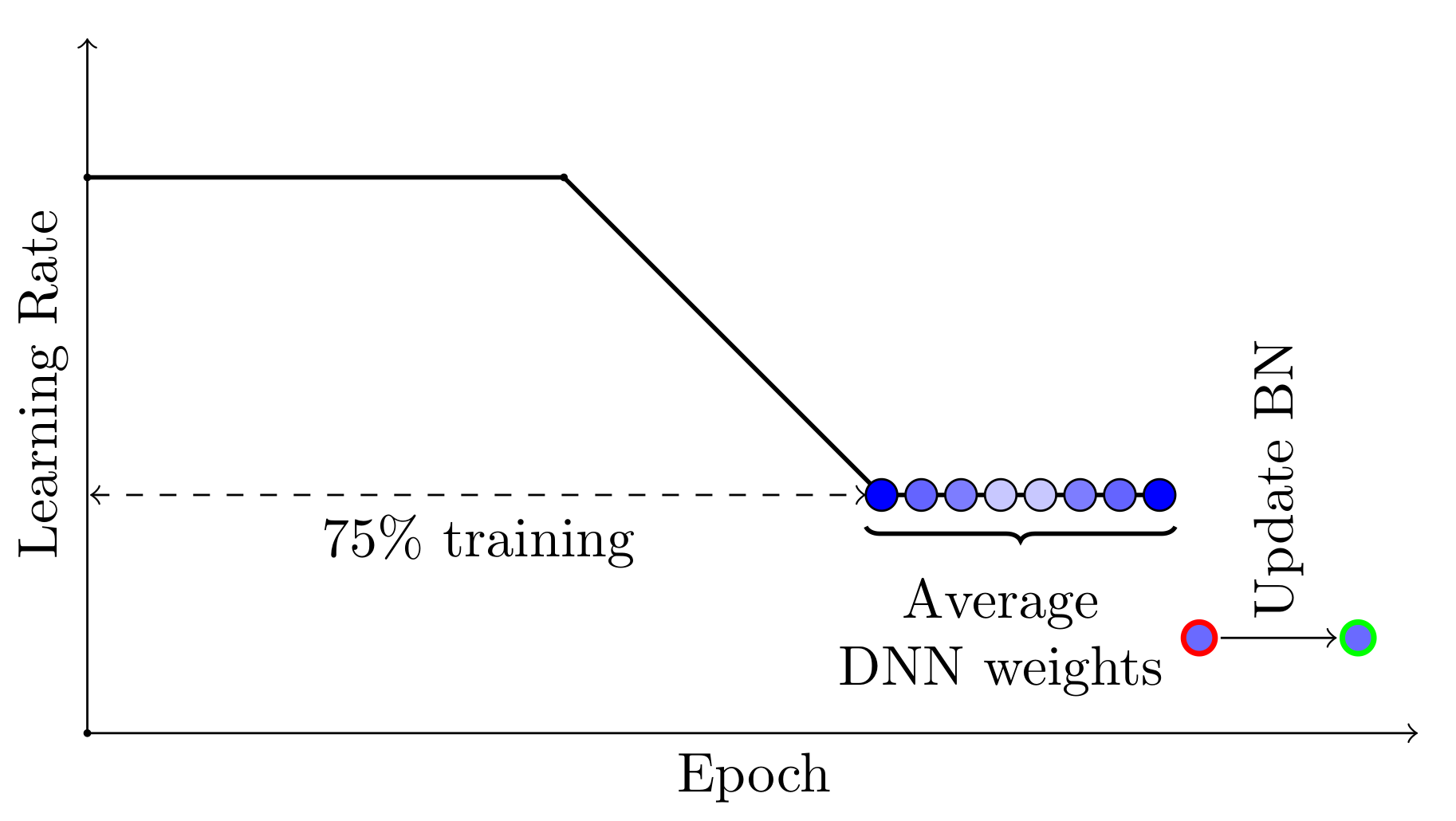
Figure 2. Illustration of the learning rate schedule adopted by SWA. Standard decaying schedule is used for the first 75% of the training and then a high constant value is used for the remaining 25%. The SWA averages are formed during the last 25% of training.
In our implementation the auto mode of the SWA optimizer allows us to run the procedure described above. To run SWA in auto mode you just need to wrap your optimizer base_opt of choice (can be SGD, Adam, or any other torch.optim.Optimizer) with SWA(base_opt, swa_start, swa_freq, swa_lr). After swa_start optimization steps the learning rate will be switched to a constant value swa_lr, and in the end of every swa_freq optimization steps a snapshot of the weights will be added to the SWA running average. Once you run opt.swap_swa_sgd(), the weights of your model are replaced with their SWA running averages.
Batch Normalization
One important detail to keep in mind is batch normalization. Batch normalization layers compute running statistics of activations during training. Note that the SWA averages of the weights are never used to make predictions during training, and so the batch normalization layers do not have the activation statistics computed after you reset the weights of your model with opt.swap_swa_sgd(). To compute the activation statistics you can just make a forward pass on your training data using the SWA model once the training is finished. In the SWA class we provide a helper function opt.bn_update(train_loader, model). It updates the activation statistics for every batch normalization layer in the model by making a forward pass on the train_loader data loader. You only need to call this function once in the end of training.
Advanced Learning-Rate Schedules
SWA can be used with any learning rate schedule that encourages exploration of the flat region of solutions. For example, you can use cyclical learning rates in the last 25% of the training time instead of a constant value, and average the weights of the networks corresponding to the lowest values of the learning rate within each cycle (see Figure 3).
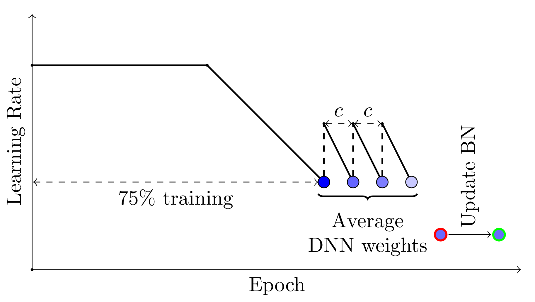
Figure 3. Illustration of SWA with an alternative learning rate schedule. Cyclical learning rates are adopted in the last 25% of training, and models for averaging are collected in the end of each cycle.
In our implementation you can implement custom learning rate and weight averaging strategies by using SWA in the manual mode. The following code is equivalent to the auto mode code presented in the beginning of this blogpost.
opt = torchcontrib.optim.SWA(base_opt)
for i in range(100):
    opt.zero_grad()
    loss_fn(model(input), target).backward()
    opt.step()
    if i > 10 and i % 5 == 0:
        opt.update_swa()
opt.swap_swa_sgd()
In manual mode you don’t specify swa_start, swa_lr and swa_freq, and just call opt.update_swa() whenever you want to update the SWA running averages (for example in the end of each learning rate cycle). In manual mode SWA doesn’t change the learning rate, so you can use any schedule you want as you would normally do with any other torch.optim.Optimizer.
Why does it work?
SGD converges to a solution within a wide flat region of loss. The weight space is extremely high-dimensional, and most of the volume of the flat region is concentrated near the boundary, so SGD solutions will always be found near the boundary of the flat region of the loss. SWA on the other hand averages multiple SGD solutions, which allows it to move towards the center of the flat region.
We expect solutions that are centered in the flat region of the loss to generalize better than those near the boundary. Indeed, train and test error surfaces are not perfectly aligned in the weight space. Solutions that are centered in the flat region are not as susceptible to the shifts between train and test error surfaces as those near the boundary. In Figure 4 below we show the train loss and test error surfaces along the direction connecting the SWA and SGD solutions. As you can see, while SWA solution has a higher train loss compared to the SGD solution, it is centered in the region of low loss, and has a substantially better test error.
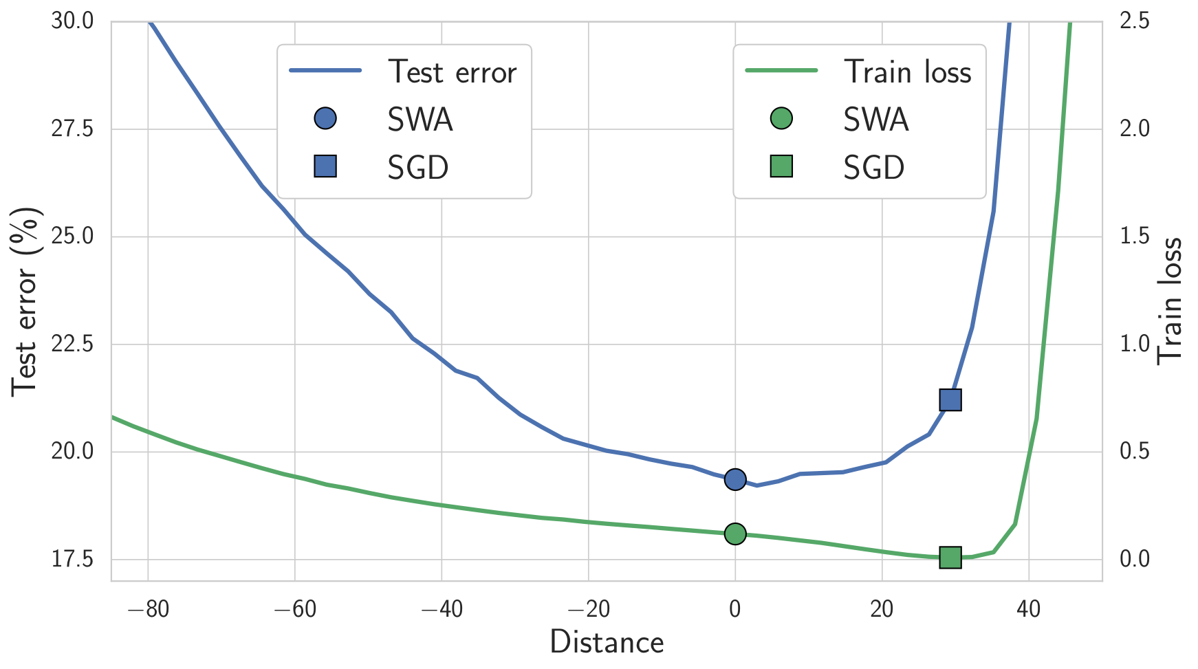
Figure 4. Train loss and test error along the line connecting the SWA solution (circle) and SGD solution (square). SWA solution is centered in a wide region of low train loss while the SGD solution lies near the boundary. Because of the shift between train loss and test error surfaces, SWA solution leads to much better generalization.
Examples and Results
We released a GitHub repo here with examples of using the torchcontrib implementation of SWA for training DNNs. For example, these examples can be used to achieve the following results on CIFAR-100:
| DNN (Budget) | SGD | SWA 1 Budget | SWA 1.25 Budgets | SWA 1.5 Budgets |
|---|---|---|---|---|
| VGG16 (200) | 72.55 ± 0.10 | 73.91 ± 0.12 | 74.17 ± 0.15 | 74.27 ± 0.25 |
| PreResNet110 (150) | 76.77 ± 0.38 | 78.75 ± 0.16 | 78.91 ± 0.29 | 79.10 ± 0.21 |
| PreResNet164 (150) | 78.49 ± 0.36 | 79.77 ± 0.17 | 80.18 ± 0.23 | 80.35 ± 0.16 |
| WideResNet28x10 (200) | 80.82 ± 0.23 | 81.46 ± 0.23 | 81.91 ± 0.27 | 82.15 ± 0.27 |
Semi-Supervised Learning
In a follow-up paper SWA was applied to semi-supervised learning, where it illustrated improvements beyond the best reported results in multiple settings. For example, with SWA you can get 95% accuracy on CIFAR-10 if you only have the training labels for 4k training data points (the previous best reported result on this problem was 93.7%). This paper also explores averaging multiple times within epochs, which can accelerate convergence and find still flatter solutions in a given time.
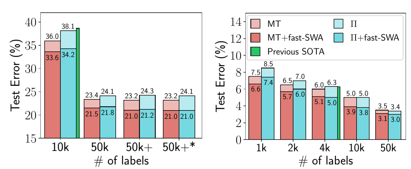
Figure 5. Performance of fast-SWA on semi-supervised learning with CIFAR-10. fast-SWA achieves record results in every setting considered.
Calibration and Uncertainty Estimates
SWA-Gaussian (SWAG) is a simple, scalable and convenient approach to uncertainty estimation and calibration in Bayesian deep learning. Similarly to SWA, which maintains a running average of SGD iterates, SWAG estimates the first and second moments of the iterates to construct a Gaussian distribution over weights. SWAG distribution approximates the shape of the true posterior: Figure 6 below shows the SWAG distribution on top of the posterior log-density for PreResNet-164 on CIFAR-100.
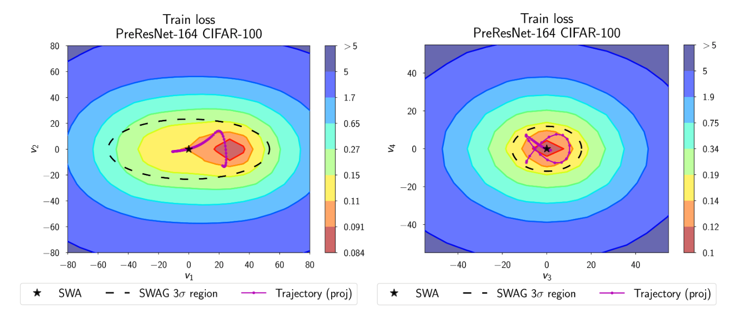
Figure 6. SWAG distribution on top of posterior log-density for PreResNet-164 on CIFAR-100. The shape of SWAG distribution is aligned with the posterior.
Empirically, SWAG performs on par or better than popular alternatives including MC dropout, KFAC Laplace, and temperature scaling on uncertainty quantification, out-of-distribution detection, calibration and transfer learning in computer vision tasks. Code for SWAG is available here.
Reinforcement Learning
In another follow-up paper SWA was shown to improve the performance of policy gradient methods A2C and DDPG on several Atari games and MuJoCo environments.
| Environment | A2C | A2C + SWA |
|---|---|---|
| Breakout | 522 ± 34 | 703 ± 60 |
| Qbert | 18777 ± 778 | 21272 ± 655 |
| SpaceInvaders | 7727 ± 1121 | 21676 ± 8897 |
| Seaquest | 1779 ± 4 | 1795 ± 4 |
| CrazyClimber | 147030 ± 10239 | 139752 ± 11618 |
| BeamRider | 9999 ± 402 | 11321 ± 1065 |
Low Precision Training
We can filter through quantization noise by combining weights that have been rounded down with weights that have been rounded up. Moreover, by averaging weights to find a flat region of the loss surface, large perturbations of the weights will not affect the quality of the solution (Figures 7 and 8). Recent work shows that by adapting SWA to the low precision setting, in a method called SWALP, one can match the performance of full-precision SGD even with all training in 8 bits [5]. This is quite a practically important result, given that (1) SGD training in 8 bits performs notably worse than full precision SGD, and (2) low precision training is significantly harder than predictions in low precision after training (the usual setting). For example, a ResNet-164 trained on CIFAR-100 with float (16-bit) SGD achieves 22.2% error, while 8-bit SGD achieves 24.0% error. By contrast, SWALP with 8 bit training achieves 21.8% error.
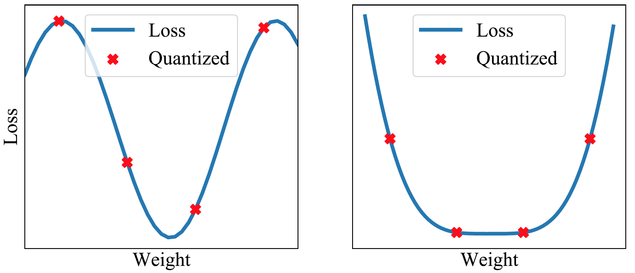
Figure 7. Quantizing in a flat region can still provide solutions with low loss.
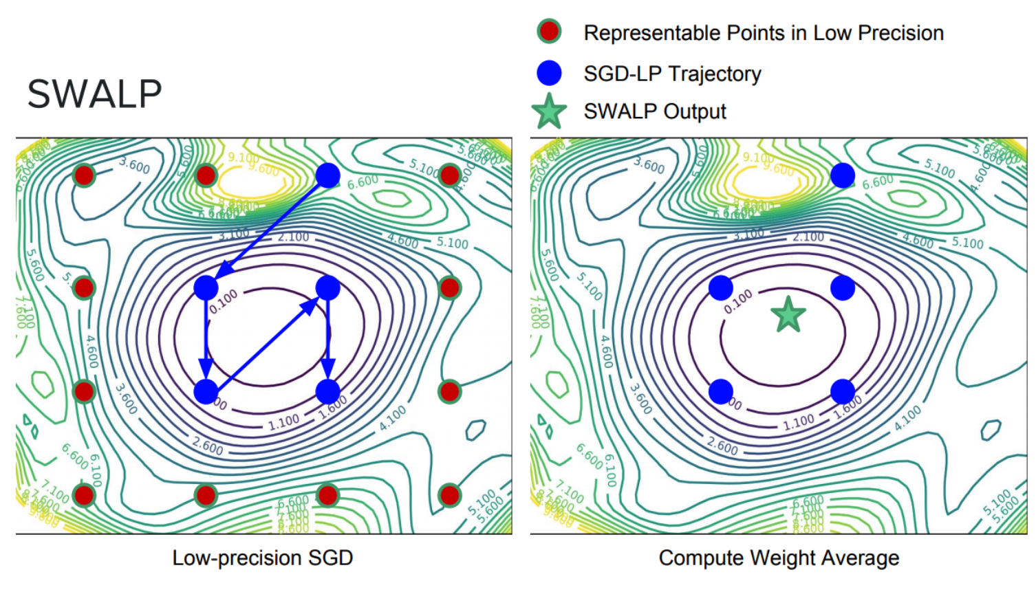
Figure 8. Low precision SGD training (with a modified learning rate schedule) and SWALP.
Conclusion
One of the greatest open questions in deep learning is why SGD manages to find good solutions, given that the training objectives are highly multimodal, and there are in principle many settings of parameters that achieve no training loss but poor generalization. By understanding geometric features such as flatness, which relate to generalization, we can begin to resolve these questions and build optimizers that provide even better generalization, and many other useful features, such as uncertainty representation. We have presented SWA, a simple drop-in replacement for standard SGD, which can in principle benefit anyone training a deep neural network. SWA has been demonstrated to have strong performance in a number of areas, including computer vision, semi-supervised learning, reinforcement learning, uncertainty representation, calibration, Bayesian model averaging, and low precision training.
We encourage you try out SWA! Using SWA is now as easy as using any other optimizer in PyTorch. And even if you have already trained your model with SGD (or any other optimizer), it’s very easy to realize the benefits of SWA by running SWA for a small number of epochs starting with a pre-trained model.
- [1] Averaging Weights Leads to Wider Optima and Better Generalization; Pavel Izmailov, Dmitry Podoprikhin, Timur Garipov, Dmitry Vetrov, Andrew Gordon Wilson; Uncertainty in Artificial Intelligence (UAI), 2018
- [2] There Are Many Consistent Explanations of Unlabeled Data: Why You Should Average; Ben Athiwaratkun, Marc Finzi, Pavel Izmailov, Andrew Gordon Wilson; International Conference on Learning Representations (ICLR), 2019
- [3] Improving Stability in Deep Reinforcement Learning with Weight Averaging; Evgenii Nikishin, Pavel Izmailov, Ben Athiwaratkun, Dmitrii Podoprikhin, Timur Garipov, Pavel Shvechikov, Dmitry Vetrov, Andrew Gordon Wilson, UAI 2018 Workshop: Uncertainty in Deep Learning, 2018
- [4] A Simple Baseline for Bayesian Uncertainty in Deep Learning, Wesley Maddox, Timur Garipov, Pavel Izmailov, Andrew Gordon Wilson, arXiv pre-print, 2019: https://arxiv.org/abs/1902.02476
- [5] SWALP : Stochastic Weight Averaging in Low Precision Training, Guandao Yang, Tianyi Zhang, Polina Kirichenko, Junwen Bai, Andrew Gordon Wilson, Christopher De Sa, To appear at the International Conference on Machine Learning (ICML), 2019.
- [6] David Ruppert. Efficient estimations from a slowly convergent Robbins-Monro process. Technical report, Cornell University Operations Research and Industrial Engineering, 1988.
- [7] Acceleration of stochastic approximation by averaging. Boris T Polyak and Anatoli B Juditsky. SIAM Journal on Control and Optimization, 30(4):838–855, 1992.
- [8] Loss Surfaces, Mode Connectivity, and Fast Ensembling of DNNs, Timur Garipov, Pavel Izmailov, Dmitrii Podoprikhin, Dmitry Vetrov, Andrew Gordon Wilson. Neural Information Processing Systems (NeurIPS), 2018
