In a landscape where AI innovation is accelerating at an unprecedented pace, Meta’s Llama family of open sourced large language models (LLMs) stands out as a notable breakthrough. Llama marked a significant step forward for LLMs, demonstrating the power of pre-trained architectures for a wide range of applications. Llama 2 further pushed the boundaries of scale and capabilities, inspiring advancements in language understanding, generation, and beyond.
Shortly after the announcement of Llama, we published a blog post showcasing ultra-low inference latency for Llama using PyTorch/XLA on Cloud TPU v4. Building on these results, today, we are proud to share Llama 2 training and inference performance using PyTorch/XLA on Cloud TPU v4 and our newest AI supercomputer, Cloud TPU v5e.
In this blog post, we use Llama 2 as an example model to demonstrate the power of PyTorch/XLA on Cloud TPUs for LLM training and inference. We discuss the computation techniques and optimizations used to improve inference throughput and training model FLOPs utilization (MFU). For Llama 2 70B parameters, we deliver 53% training MFU, 17 ms/token inference latency, 42 tokens/s/chip throughput powered by PyTorch/XLA on Google Cloud TPU. We offer a training user guide and an inference user guide for reproducing the results in this article. Additionally, you may find our Google Next 2023 presentation here.
Model Overview
Llama 2 comes in various sizes, ranging from 7B to 70B parameters, catering to different needs, computational resources, and training / inference budgets. Whether it’s small-scale projects or large-scale deployments, Llama models offer versatility and scalability to accommodate a wide range of applications.
Llama 2 is an auto-regressive language model that uses an optimized transformer architecture. The largest, 70B model, uses grouped-query attention, which speeds up inference without sacrificing quality. Llama 2 is trained on 2 trillion tokens (40% more data than Llama) and has the context length of 4,096 tokens for inference (double the context length of Llama), which enables more accuracy, fluency, and creativity for the model.
Llama 2 is a state-of-the-art LLM that outperforms many other open source language models on many benchmarks, including reasoning, coding, proficiency, and knowledge tests. The model’s scale and complexity place many demands on AI accelerators, making it an ideal benchmark for LLM training and inference performance of PyTorch/XLA on Cloud TPUs.
Performance Challenge of LLMs
Large-scale distributed training for LLMs such as Llama 2 introduces technical challenges that require practical solutions to make the most efficient use of TPUs. Llama’s size can strain both memory and processing resources of TPUs. To address this, we use model sharding, which involves breaking down the model into smaller segments, each fitting within the capacity of a single TPU core. This enables parallelism across multiple TPUs, improving training speed while reducing communication overhead.
Another challenge is managing the large datasets required for training Llama 2 efficiently, which requires effective data distribution and synchronization methods. Additionally, optimizing factors like learning rate schedules, gradient aggregation, and weight synchronization across distributed TPUs is crucial for achieving convergence.
After pretraining or fine-tuning Llama 2, running inference on the model checkpoint creates additional technical challenges. All of the challenges discussed in our previous blog post, such as autoregressive decoding, variable input prompt lengths, and the need for model sharding and quantization still apply for Llama 2. In addition, Llama 2 introduced two new capabilities: grouped-query attention and early stopping. We discuss how PyTorch/XLA handles these challenges to enable high-performance, cost-efficient training and inference of Llama 2 on Cloud TPU v4 and v5e.
Large-Scale Distributed Training
PyTorch/XLA offers two major ways of doing large-scale distributed training: SPMD, which utilizes the XLA compiler to transform and partition a single-device program into a multi-device distributed program; and FSDP, which implements the widely-adopted Fully Sharded Data Parallel algorithm.
In this blog post, we show how to use the SPMD API to annotate the HuggingFace (HF) Llama 2 implementation to maximize performance. For comparison, we also show our FSDP results with the same configurations; read about PyTorch/XLA FSDP API here.
SPMD Overview
Let’s briefly review the fundamentals of SPMD. For details, please refer to our blog post and user guide.
Mesh
A multidimensional array that describes the logical topology of the TPU devices:
# Assuming you are running on a TPU host that has 8 devices attached
num_devices = xr.global_runtime_device_count()
# mesh shape will be (4,2) in this example
mesh_shape = (num_devices // 2, 2)
device_ids = np.array(range(num_devices))
# axis_names 'x' and 'y' are optional
mesh = Mesh(device_ids, mesh_shape, ('x', 'y'))
Partition Spec
A tuple that describes how the corresponding tensor’s dimensions are sharded across the mesh:
partition_spec = ('x', 'y')
Mark Sharding
An API that takes a mesh and a partition_spec, and then generates a sharding annotation for the XLA compiler.
tensor = torch.randn(4, 4).to('xla')
# Let's resue the above mesh and partition_spec.
# It means the tensor's 0th dim is sharded 4 way and 1th dim is sharded 2 way.
xs.mark_sharding(tensor, mesh, partition_spec)
2D Sharding with SPMD
In our SPMD blog post, we demonstrated using 1D FSDP style sharding. Here, we introduce a more powerful sharding strategy, called 2D sharding, where both the parameters and activations are sharded. This new sharding strategy not only allows fitting a larger model but also boosts the MFU to up to 54.3%. For more details, read the Benchmarks section.
This section introduces a set of general rules that applies to most LLMs, and for convenience we directly reference the variable names and configuration names from HF Llama.
First, let’s create a 2D Mesh with corresponding axis names: data and model. The data axis is usually where we distribute the input data, and the model axis is where we further distribute the model.
mesh = Mesh(device_ids, mesh_shape, ('data', 'model'))
The mesh_shape can be a hyper-parameter that is tuned for different model sizes and hardware configurations. The same mesh will be reused in all following sharding annotations. In the next few sections, we will cover how to use the mesh to shard parameters, activations and input data.
Parameter Sharding
Below is a table that summarizes all parameters of HF Llama 2 and corresponding partition specifications. Example HF code can be found here.
| Parameter Name | Explanation | Parameter Shape | Partition Spec |
embed_tokens | embedding layer | (vocab_size, hidden_size) | (model, data) |
q_proj | attention weights | (num_heads x head_dim, hidden_size) | (data, model) |
k_proj / v_proj | attention weights | (num_key_value_heads x head_dim, hidden_size) | (data, model) |
o_proj | attention weights | (hidden_size, num_heads x head_dim) | (model, data) |
gate_proj / up_proj | MLP weights | (intermediate_size, hidden_size) | (model, data) |
down_proj | MLP weights | (hidden_size, intermediate_size) | (data, model) |
lm_head | HF output embedding | (vocab_size, hidden_size) | (model, data) |
Table 1: SPMD 2D Sharding Parameter Partition Spec
The rule is to shard the hidden_size dim of any weights except QKVO projections according to the data axis of the mesh, then shard the other dim with the remaining model axis. For QKVO, do the opposite. This model-data axis rotation methodology is similar to that of Megatron-LM to reduce communication overhead. For layernorm weights, we implicitly mark them as replicated across different devices given they are 1D tensors.
Activation Sharding
In order to better utilize the device memory, very often we need to annotate the output of some memory bound ops. That way the compiler is forced to only keep partial output on devices instead of the full output. In Llama 2, we explicitly annotate all torch.matmul and nn.Linear outputs. Table 2 summarizes the corresponding annotations; the example HF code can be found here.
| Output Name | Explanation | Output Shape | Partition Spec |
inputs_embeds | embedding layer output | (batch_size, sequence_length, hidden_size) | (data, None, model) |
query_states | attention nn.Linear output | (batch_size, sequence_length, num_heads x head_dim) | (data, None, model) |
key_states / value_states | attention nn.Linear output | (batch_size, sequence_length, num_key_value_heads x head_dim) | (data, None, model) |
attn_weights | attention weights | (batch_size, num_attention_heads, sequence_length, sequence_length) | (data, model, None, None) |
attn_output | attention layer output | (batch_size, sequence_length, hidden_size) | (data, None, model) |
up_proj / gate_proj / down_proj | MLP nn.Linear outputs | (batch_size, sequence_length, intermediate_size) | (data, None, model) |
logits | HF output embedding output | (batch_size, sequence_length, hidden_size) | (data, None, model) |
Table 2: SPMD 2D Sharding Activation Partition Spec
The rule is to shard the batch_size dim of any outputs according to the data axis of the mesh, then replicate the length dims of any outputs, and finally shard the last dim along the model axis.
Input Sharding
For input sharding, the rule is to shard the batch dim along the data axis of the mesh, and replicate the sequence_length dim. Below is the example code, and the corresponding HF change may be found here.
partition_spec = ('data', None)
sharding_spec = xs.ShardingSpec(mesh, partition_spec)
# MpDeviceLoader will shard the input data before sending to the device.
pl.MpDeviceLoader(dataloader, self.args.device, input_sharding=sharding_spec, ...)
Now, all the data and model tensors that require sharding are covered!
Optimizer States & Gradients
You may be wondering whether it is necessary to shard the optimizer states and gradients as well. Great news: the sharding propagation feature of the XLA compiler automates the sharding annotation in these two scenarios, without needing more hints to improve performance.
It is important to note that optimizer states are typically initialized within the first iteration of the training loop. From the standpoint of the XLA compiler, the optimizer states are the outputs of the first graph, and therefore have the sharding annotation propagated. For subsequent iterations, the optimizer states become inputs to the second graph, with the sharding annotation propagated from the first one. This is also why PyTorch/XLA typically produces two graphs for the training loops. If the optimizer states are somehow initialized before the first iteration, users will have to manually annotate them, just like the model weights.
Again, all concrete examples of the above sharding annotation can be found in our fork of HF Transformers here. The repo also contains code for our experimental feature MultiSlice, including HybridMesh and dcn axis, which follows the same principles mentioned above.
Caveats
While using SPMD for training, there are a few important things to pay attention to:
- Use
torch.einsuminstead oftorch.matmul;torch.matmulusually flattens tensors and does atorch.mmat the end, and that’s bad for SPMD when the combined axes are sharded. The XLA compiler will have a hard time determining how to propagate the sharding. - PyTorch/XLA provides patched
[nn.Linear](https://github.com/pytorch/xla/blob/master/torch_xla/experimental/xla_sharding.py#L570)to overcome the above constraint:
import torch_xla.experimental.xla_sharding as xs
from torch_xla.distributed.fsdp.utils import apply_xla_patch_to_nn_linear

 model = apply_xla_patch_to_nn_linear(model, xs.xla_patched_nn_linear_forward)
- Always reuse the same mesh across all shardings
- Always specify
--dataloader_drop_last yes. The last smaller data is hard to annotate. - Large models which are initialized on the host can induce host-side OOM. One way to avoid this issue is to initialize parameters on the meta device, then create and shard real tensors layer-by-layer.
Infrastructure Improvements
Besides the above modeling techniques, we have developed additional features and improvements to maximize performance, including:
- We enable asynchronous collective communication. This requires enhancements on the XLA compiler’s latency hiding scheduler to better optimize for the Llama 2 PyTorch code.
- We now allow sharding annotations in the middle of the IR graph, just like JAX’s jax.lax.with_sharding_constraint. Previously, only graph inputs were annotated.
- We also propagate replicated sharding spec from the compiler to the graph outputs. This allows us to shard the optimizer states automatically.
Inference Optimizations
All the PyTorch/XLA optimizations implemented for Llama inference are applied to Llama 2 as well. That includes Tensor Parallelism + Dynamo (torch.compile) using torch-xla collective ops, autoregressive decoding logic improvement to avoid recompilation, bucketized prompt length, KV-cache with compilation friendly index ops. Llama 2 introduces two new changes: Grouped Query Attention, and Early Stopping when eos is reached for all prompts. We applied corresponding changes to promote better performance and flexibility with PyTorch/XLA.
Grouped Query Attention
Llama 2 enables Grouped Query Attention for the 70B models. It allows the number of Key and Value heads to be smaller than the number of Query heads, while still supporting KV-cache sharding up to the number of KV heads. For the 70B models, the n_kv_heads is 8, which limits the tensor parallelism to be less or equal to 8. In order to shard the model checkpoint to run on more devices, the K, V projection weights need to be replicated first, and then split into multiple pieces. For example, to shard the 70B model checkpoint from 8 pieces to 16 pieces, the K, V projection weights are duplicated and split into 2 pieces for each shard. We provide a reshard_checkpoints.py script to handle that, and to make sure the sharded checkpoint performs mathematically identical to the original checkpoint.
EOS Early Stopping
The Llama 2 generation code added the early stopping logic. A eos_reached tensor is used to track the completion of all the prompt generations, and if the eos token is reached for all the prompts in the batch, the generation would stop early. The similar change is incorporated in the PyTorch/XLA optimized version as well, with some minor tweaks.
In PyTorch/XLA, checking the value of a tensor like eos_reached as part of the control flow condition would invoke a blocking device-to-host transfer. The tensor would be transferred from device memory to CPU memory to evaluate its value, while all other logics are waiting. This introduced a delay on the scale of ms after every new token generation. As a trade-off, we reduce the rate of checking the eos_reached value to be once every 10 new token generations. With this change, the impact of the blocking device-to-host transfer would be reduced by 10x, while the early stopping would still be effective, and at most 9 unnecessary tokens would be generated after each sequence reaches the eos token.
Model Serving
PyTorch/XLA is working on a serving strategy to enable the PyTorch community to serve their deep learning applications via Torch.Export, StableHLO, and SavedModel. PyTorch/XLA Serving is an experimental feature in PyTorch/XLA 2.1 release; for details visit our serving user guide. Users can take advantage of TorchServe to run their single-host workloads.
Benchmarks
Metrics
To measure training performance, we use the industry-standard metric: Model FLOPS Utilization (MFU). Model FLOPS are the floating point operations required to perform a single forward and backward pass. Model FLOPs are hardware and implementation independent and only depend on the underlying model. MFU measures how effectively the model is using the actual hardware during training. Achieving 100% MFU means that the model is using the hardware perfectly.
To measure inference performance, we use the industry-standard metric of throughput. First, we measure latency per token when the model has been compiled and loaded. Then, we calculate throughput by dividing batch size (BS) over latency per chip. As a result, throughput measures how the model is performing in production environments regardless of how many chips are used.
Results
Training Evaluation
Figure 1 shows Llama 2 SPMD 2D sharding training results on a range of Google TPU v4 hardware with PyTorch/XLA FSDP as the baseline. We increased MFU by 28% across all sizes of Llama 2 compared to FSDP running on the same hardware configuration. This performance improvement is largely due to: 1) 2D Sharding has less communication overhead than FSDP, and 2) asynchronous collective communication is enabled in SPMD which allows communication and computation overlapping. Also note that as the model size scales, we maintain the high MFU. Table 3 shows all the hardware configurations plus some hyperparameters used in the training benchmarks.
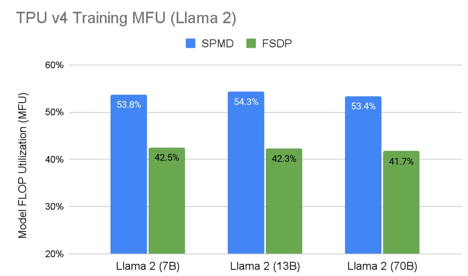
Fig. 1: Llama 2 Training MFU on TPU v4 Hardware
The results in Figure 1 are produced with sequence length 1,024. Figure 2 shows how the performance behaves with larger sequence lengths. It shows our performance also scales linearly with sequence lengths. The MFU is expected to decrease a little as a smaller per device batch size is needed to accommodate the additional memory pressure introduced by the larger sequence length since the sequence length axis is not sharded in 2D sharding. And TPU is very sensitive to batch size. For Llama 2, 70B parameters, the performance decrease is as low as 4%. At the time of preparing these results, Hugging Face Llama 2 tokenizer limits the max model input to 2,048, preventing us from evaluating larger sequence lengths.
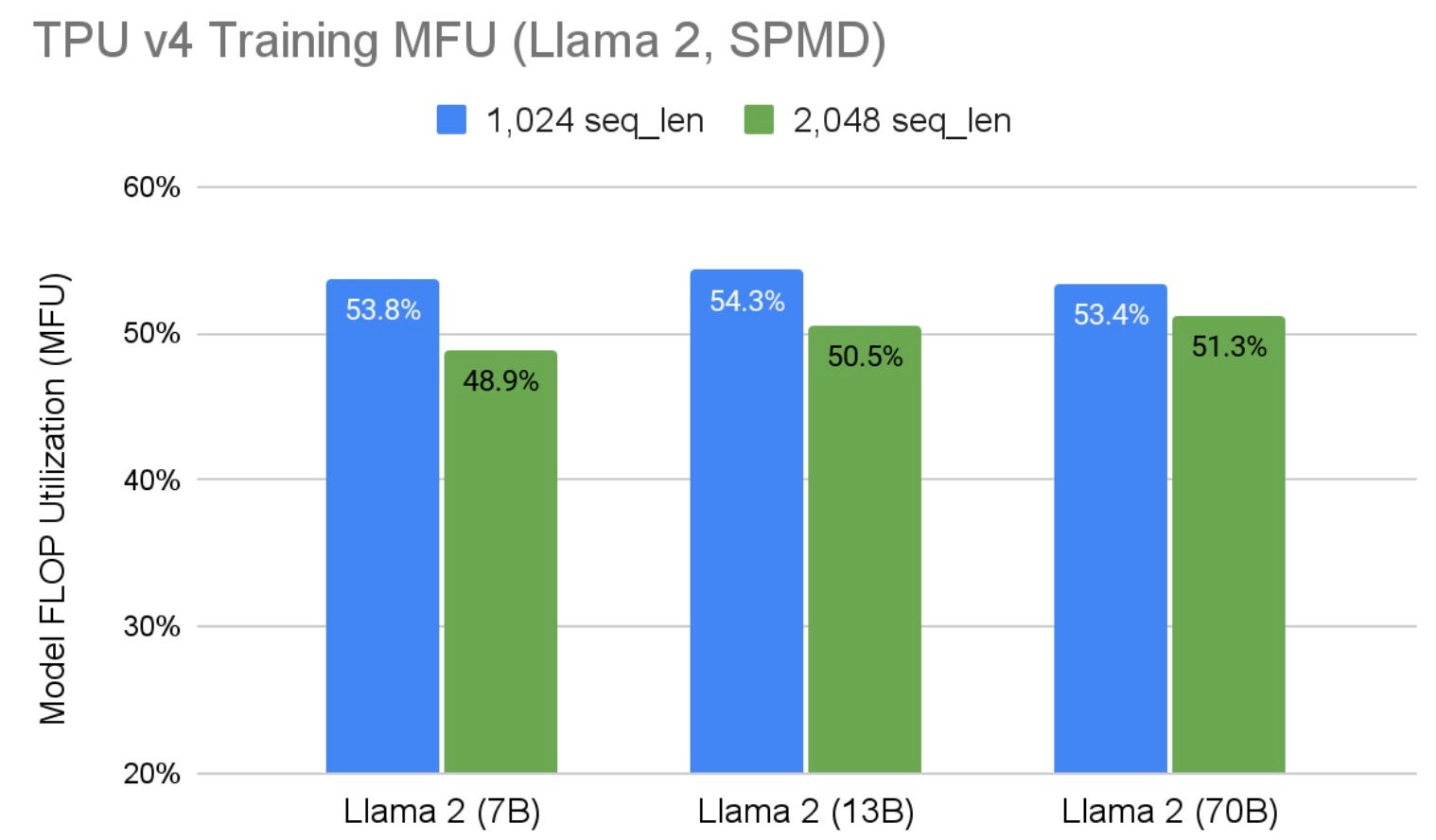
Fig. 2: Llama 2 SPMD Training MFU on TPU v4 with Different Sequence Lengths
| Model Size | 7B | 13B | 70B | |||
| TPU NumCores | V4-32 | V4-64 | V4-256 | |||
| Mesh Shape | (16, 1) | (32, 1) | (32, 4) | |||
| Seq Len | 1,024 | 2,048 | 1,024 | 2,048 | 1,024 | 2,048 |
| Global Batch | 256 | 128 | 256 | 128 | 512 | 256 |
| Per Device Batch | 16 | 8 | 8 | 4 | 16 | 8 |
Table 3: Llama 2 SPMD Training Benchmark TPU Configurations and Hyperparameters
One last thing to call out is that we use adafactor as the optimizer for better memory utilization. And once again, here is the user guide to reproduce the benchmark results listed above.
Inference Evaluation
In this section, we extend our previous evaluation of Llama on Cloud v4 TPU. Here, we demonstrate the performance properties of TPU v5e for inference applications.
We define inference throughput as the number of tokens produced by a model per second per TPU chip. Figure 3 shows Llama 2 70B throughput on a v5e-16 TPU node. Given Llama is a memory bound application, we see that applying weight-only quantization unblocks extending the model batch size to 32. Higher throughput results would be possible on larger TPU v5e hardware up to the point where the ICI network bandwidth between chips throttle the TPU slice from delivering higher throughput. Exploring the upper bound limits of TPU v5e on Llama 2 was outside of the scope of this work. Notice, to make the Llama 2 70B model run on v5e-16, we replicated the attention heads to have one head per chip as discussed in the Inference section above. As discussed previously, with increasing model batch size, per-token latency grows proportionally; quantization improves overall latency by reducing memory I/O demand.
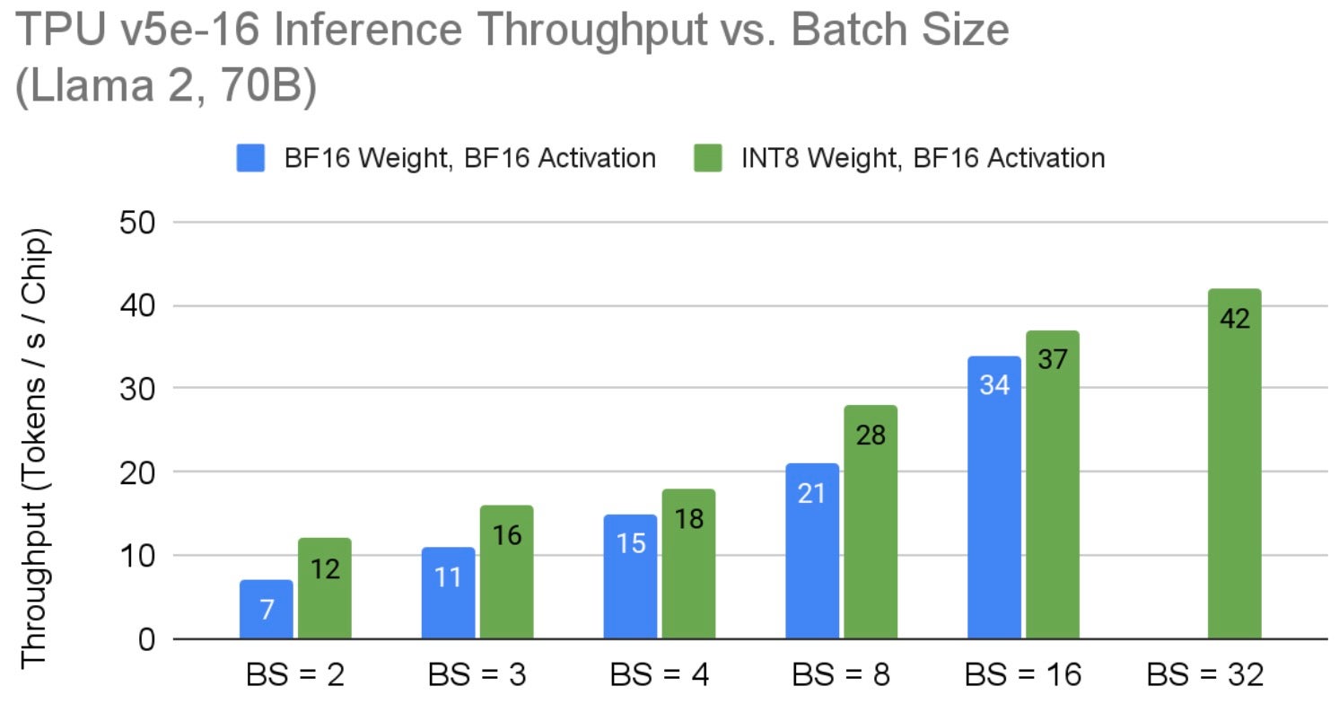
Fig. 3: Llama 2 70B Inference Per-Chip Throughput on TPU v5e vs. Batch Size
Figure 4 shows inference throughput results across different model sizes. These results highlight the largest throughput given the hardware configuration when using bf16 precision. With weight only quantization, this throughput reaches 42 on the 70B model. As mentioned above, increasing hardware resources may lead to performance gains.
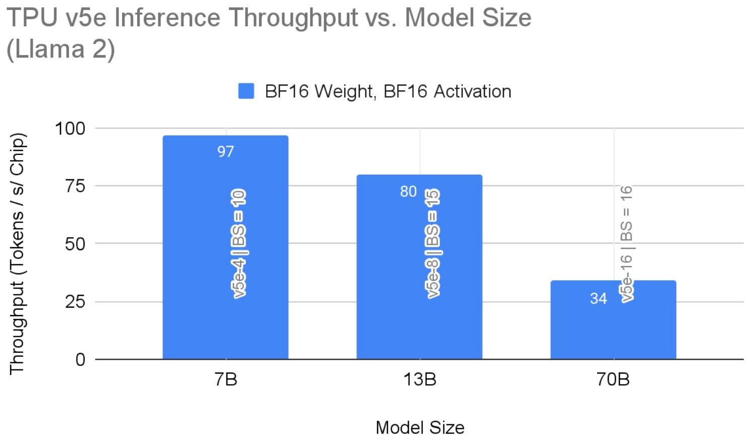
Fig. 4: Llama 2 Inference Per-Chip Throughput on TPU v5e
Figure 5 shows the cost of serving Llama 2 models (from Figure 4) on Cloud TPU v5e. We report the TPU v5e per-chip cost based on the 3-year commitment (reserved) price in the us-west4 region. All model sizes use maximum sequence length of 2,048 and maximum generation length of 1,000 tokens. Note that with quantization, the cost for the 70B model drops to $0.0036 per 1,000 tokens.
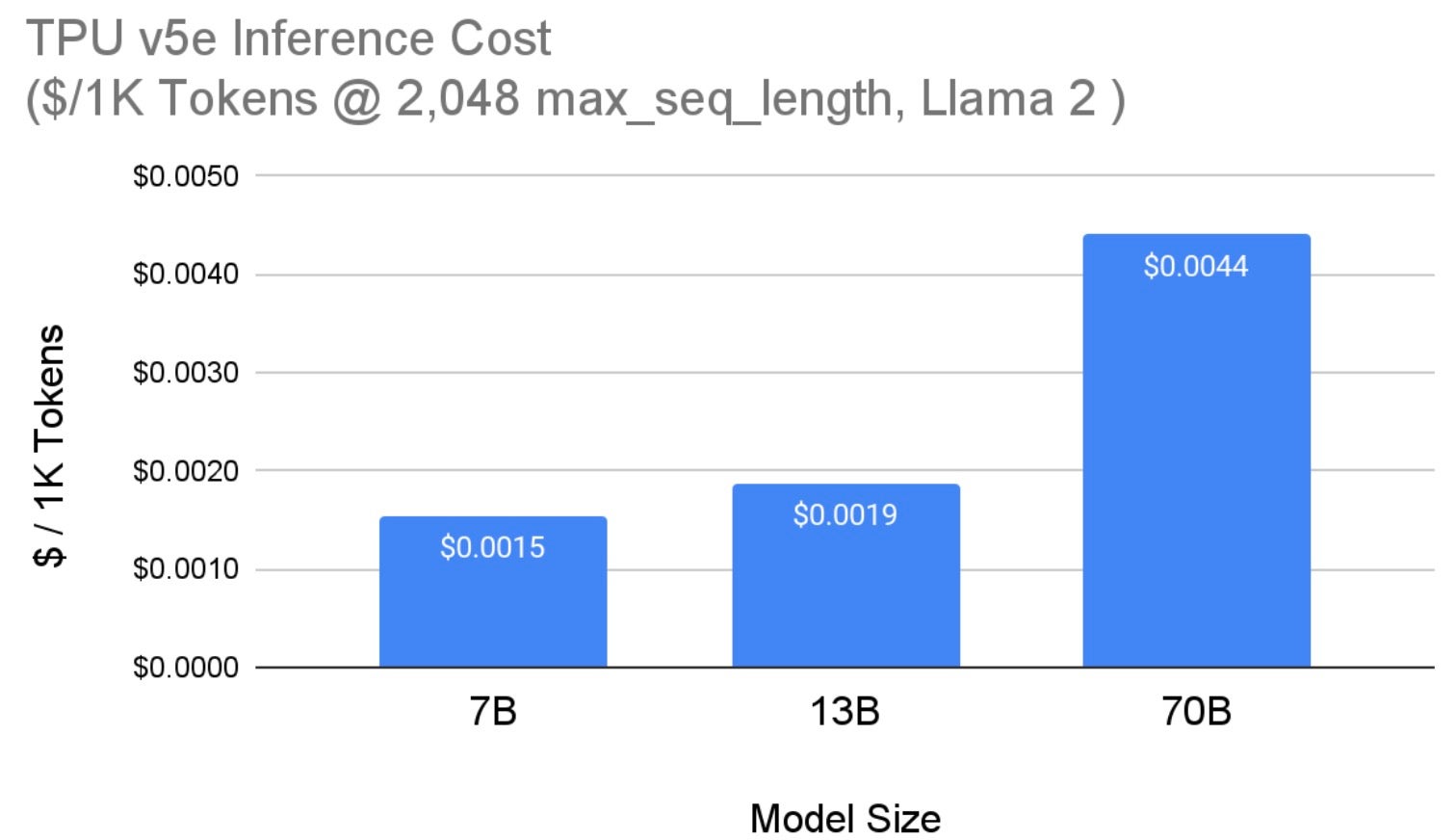
Fig. 5: Llama 2 Inference Per-Chip Cost on TPU v5e
Figure 6 summarizes our best Llama 2 inference latency results on TPU v5e. Llama 2 7B results are obtained from our non-quantized configuration (BF16 Weight, BF16 Activation) while the 13B and 70B results are from the quantized (INT8 Weight, BF16 Activation) configuration. We attribute this observation to the inherent memory saving vs. compute overhead tradeoff of quantization; as a result, for smaller models, quantization may not lead to lower inference latency.
Additionally, prompt length has a strong effect on the memory requirements of LLMs. For instance, we observe a latency of 1.2ms / token (i.e. 201 tokens / second / chip) when max_seq_len=256 at batch size of 1 with no quantization on v5e-4 running Llama2 7B.
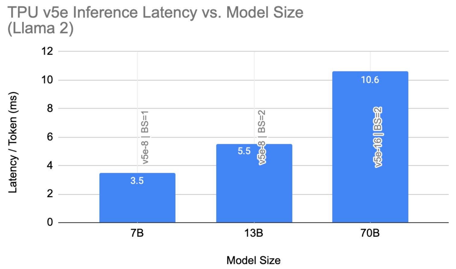
Fig. 6: Llama 2 Inference Latency on TPU v5e
Final Thoughts
The recent wave of AI innovation has been nothing short of transformative, with breakthroughs in LLMs at the forefront. Meta’s Llama and Llama 2 models stand as notable milestones in this wave of progress. PyTorch/XLA uniquely enables high-performance, cost-efficient training and inference for Llama 2 and other LLMs and generative AI models on Cloud TPUs, including the new Cloud TPU v5e. Looking forward, PyTorch/XLA will continue to push the performance limits on Cloud TPUs in both throughput and scalability and at the same time maintain the same PyTorch user experience.
We are ecstatic about what’s ahead for PyTorch/XLA and invite the community to join us. PyTorch/XLA is developed fully in open source. So, please file issues, submit pull requests, and send RFCs to GitHub so that we can openly collaborate. You can also try out PyTorch/XLA for yourself on various XLA devices including TPUs and GPUs.
We would like to extend our special thanks to Marcello Maggioni, Tongfei Guo, Andy Davis, Berkin Ilbeyi for their support and collaboration in this effort.
Cheers,
The PyTorch/XLA Team at Google