TL;DR
Leveraging a first principles approach, we showcase a step by step process undertaken to accelerate the current Triton GPTQ kernels by 3x (core GPTQ) and 6x (AutoGPTQ). Example: 275us to 47us on a typical Llama style inference input. The goal is to provide a helpful template for accelerating any given Triton kernel. We provide a background on Triton and GPTQ quantization and dequantization process, showcase the impact of coalesced memory access to improve shared and global memory throughput, highlight changes made to reduce warp stalling to improve total throughput, and an overview on integrating Triton kernels into PyTorch code. Longer term, we hope to surpass the existing CUDA native GPTQ kernel with our Triton kernel.
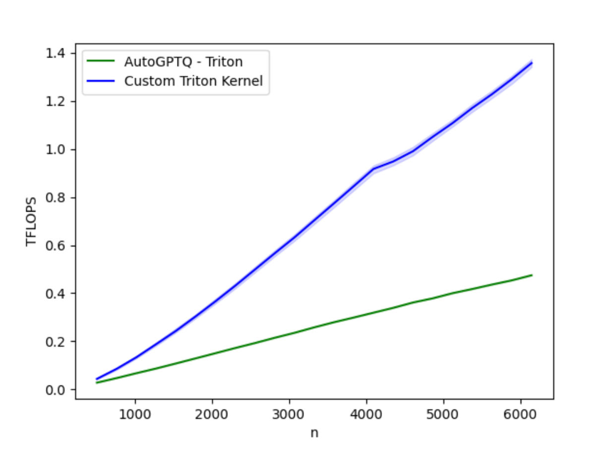
Fig 1: Performance benchmarking the optimized AutoGTPQ kernel vs the current AutoGPTQ kernel on H100
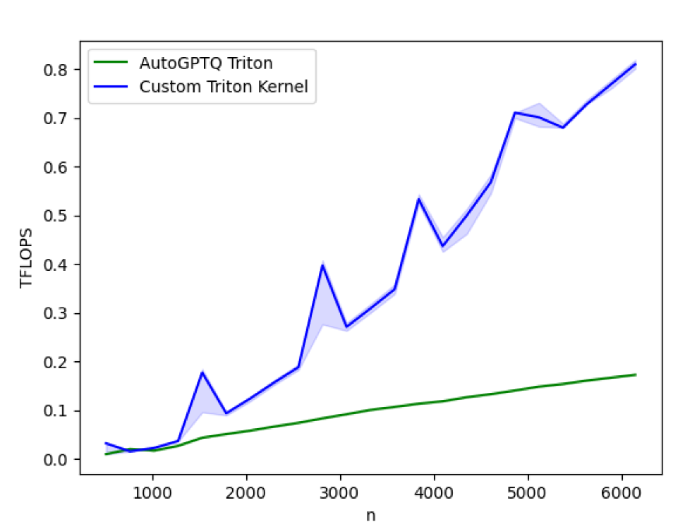
Fig 2: Performance benchmarking the newly optimized AutoGTPQ kernel vs the current AutoGPTQ kernel on A100
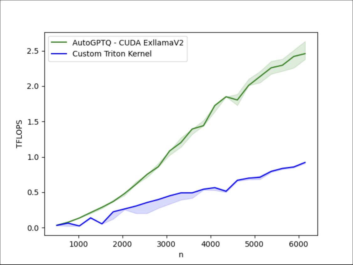
Fig 3: Even with these improvements, there remains a gap between our optimized Triton kernel and the CUDA native AutoGTPQ kernel on A100. More to come…
1.0 Introduction to Triton
The Triton framework provides a hardware agnostic way of programming and targeting GPUs, currently supporting both NVIDIA and AMD, with support for additional hardware vendors in progress. Triton is now a mainstay for PyTorch 2.0 as torch.compile decomposes eager PyTorch and re-assembles it into a high percentage of Triton kernels with PyTorch connecting code.
As Triton becomes more widely adopted, it will be essential that programmers understand how to systematically step through the Triton stack (from the high level Python down to the low-level SASS) to address performance bottlenecks in order to optimize GPU efficiency for algorithms that go beyond torch.compile generated kernels.
In this post, we will introduce some core concepts of the Triton programming language, how to identify common performance limiters in GPU kernels, and in parallel, tune a quantization kernel used in AutoGPTQ that can be used for high throughput inference applications.
Intro to GPTQ Quantization and Dequantization
GPTQ is a quantization algorithm that is able to compress ultra-large (175B+) LLMs efficiently to int4 bit representation, via approximate second order information (Hessian inverse). AutoGPTQ is a framework built on GPTQ, allowing for rapid dequantization and inference/serving of LLMs that have been quantized with GPTQ.
As part of the AutoGPTQ stack, they provide a Triton GPTQ kernel to handle the dequantization of a model for inference.
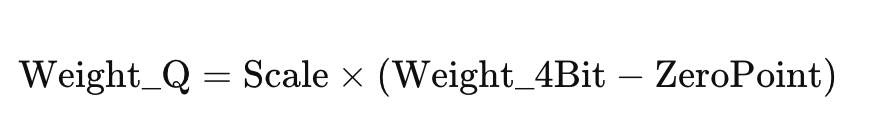
The basic process for INT quantization is shown below and involves determining the scale and zero point, and then computing the quantized 4bit Weight using the Scale and Zero point:
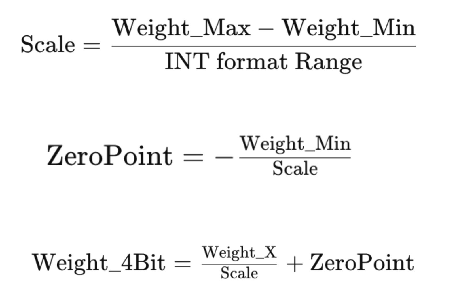
We thus store the 4 Bit weights along with the meta information of Scale and ZeroPoint for each group of weights.
To ‘dequant’ these weights, we do the following:
And then proceed to Matrix Multiply the dequantized weights with the dense input feature matrix for this linear layer.
2.0 Identify the Bottlenecks – Optimizing Matrix Multiplication
As it turns out, making a fast matrix multiplication kernel is not trivial. A naively implemented matrix multiply will rarely reach peak throughput performance on highly parallel machines like GPUs. So – we need to tackle our compute and memory subsystems in our GPU in an hierarchical fashion to make sure we are maximally utilizing each resource.
We start our optimization process, by running the unoptimized Triton Kernel, through the Nvidia Nsight Compute tool and taking a note of some important metrics and warnings:
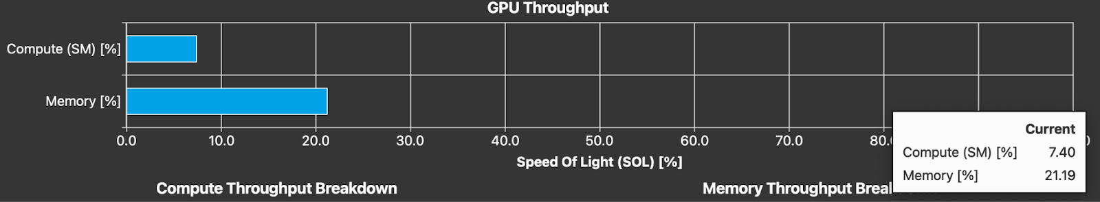
Fig xy (todo)

We notice first that both compute and memory throughput are low, 7.40% and 21.19% respectively (fig xy) . Knowing that for typical inference matrix problem sizes, we are in the memory bound regime, we will attempt to optimize the kernel by applying code changes that target the memory subsystem of our A100 GPU.
The three topics this post will cover are:
- L2 Optimization
- Vectorized Load
- Warp Stalling
Let’s walk through each topic, make the appropriate changes, and see its corresponding impact on our Triton Kernel. This Triton kernel is a fused dequantization kernel that dequantizes a packed int32 weight (we will refer to this as the B Matrix) Tensor into int4 weights, performs matrix multiplication with the activation tensor (refer to as the A matrix) in FP16 mode, and then stores the results back to a matrix C.
The above is referred to as W4A16 quantization. Keep in mind that the process we describe can and should be used for the development of any GPU kernel, as these are common bottlenecks in any unoptimized kernel.
3.0 L2 Optimization
This optimization already exists in the AutoGPTQ kernel, but we’d like to dedicate a section to this to help readers better understand how mapping and execution order of thread blocks is handled in Triton. Thus, we will step through a naive mapping and then a more optimal mapping to see its corresponding impact.
Let’s build up our kernel naively, starting with a “linear” load from global memory and then compare it to a more optimized “swizzled” load. Linear vs Swizzled determines the execution order of our grid of work on the GPU. Let’s take a look at the hints that the Nvidia Nsight Compute Tool provides regarding our kernels shared memory access pattern in the naive case:
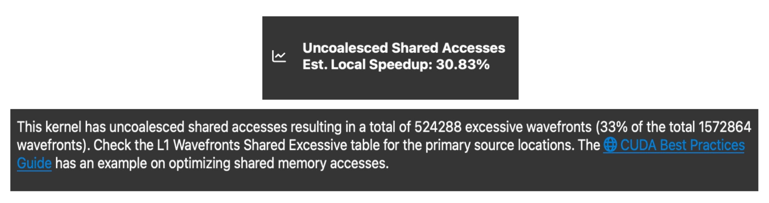
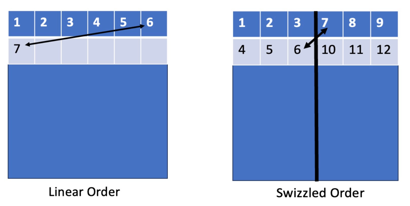
To tackle this issue we can use an approach referred to as “tile-swizzling.” The idea of this method is to launch our thread blocks in a more L2 cache friendly order.
Let’s take a step back and familiarize ourselves with some Triton semantics and make a simple CUDA analogy to understand the concept better. Triton kernels launch “programs”. These so-called programs map to the concept of a Thread Block in CUDA and it is the basic unit of parallelism in a Triton Kernel. Every program has with it associated a “pid” and all the threads in a program are guaranteed to be executing the same instruction.
The Triton programs will be distributed onto your SMs in a naive-way if you do a simple linear mapping of “pid” to a 2D grid location of your output matrix C.
This 2D grid location is determined by pid_m and pid_n in Triton. We would like to exploit data and cache locality in the L2 cache of our GPU, when we distribute our grid of work. To do this in Triton we can make the following changes:
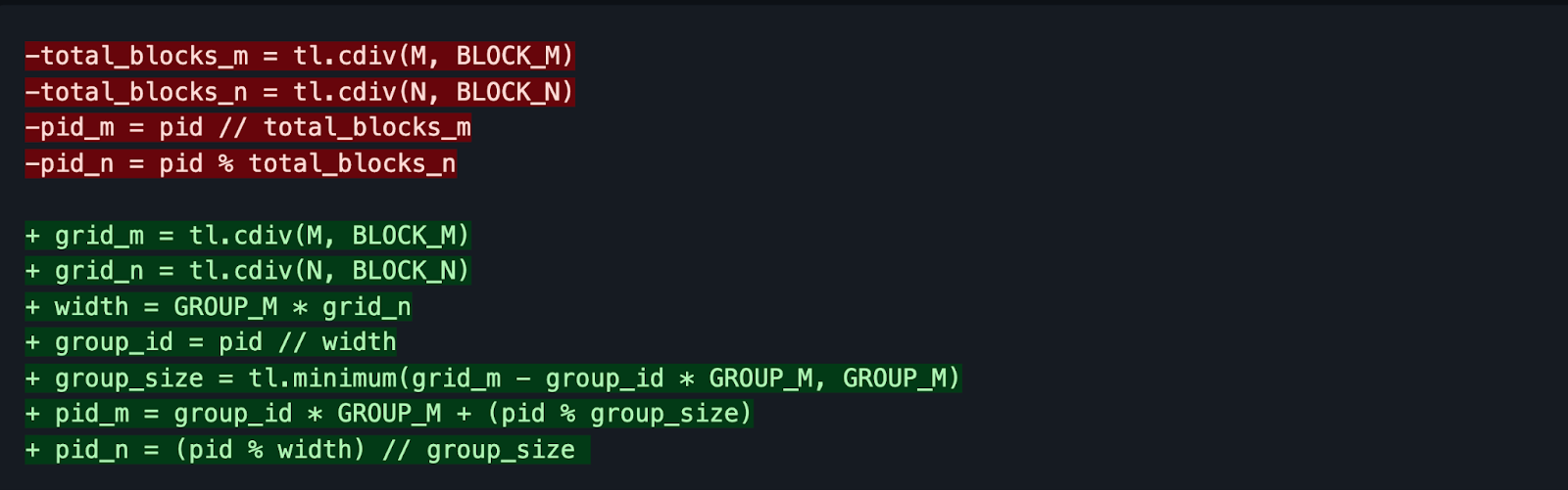
The code highlighted in red would be the naive “linear” tile ordering, and the code highlighted in green is the “swizzled” tile ordering. This type of launch promotes a sense of locality. Here is a visual to help understand this better.
After incorporating this change, the profiler no longer complains about uncoalesced memory accesses. Let’s take a look at how our memory throughput has changed:
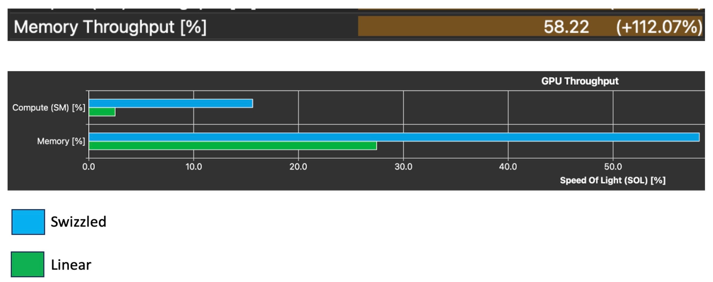
This change was tested on a simple load store kernel. Looking at the GPU speed of light statistics section in the profiler we also see a 112.07% increase in the memory throughput of the simple load kernel, which is what we were after with this optimization. Again, this optimization already exists in the AutoGPTQ kernel, but is the boilerplate logic that every Triton Kernel programmer will have to write in the beginning of their kernel, before any of the exciting dequantization or matrix multiply logic. It is thus important to understand that:
- This mapping is not unique
- Triton does not automatically handle this kind of optimization for the programmer, and careful thought must be taken to ensure your kernel is optimally handling shared memory accesses
These are not obvious for those new to Triton, as much of the shared memory access optimization is handled by the Triton compiler. However, in the cases where these are not handled by the compiler, it is important to be able to understand what tools and methods are available to us to be able to influence memory behavior.
4.0 Vectorized Load
Now, back to the original complaints of our unoptimized kernel. We want to optimize the global memory access pattern of our kernel. From the details page of the Nvidia Nsight compute tool, we see the following note, where the profiler is complaining about uncoalesced global memory accesses.
Let’s dig deeper and take a look at the SASS (Assembly) Code load for an unoptimized memory read:
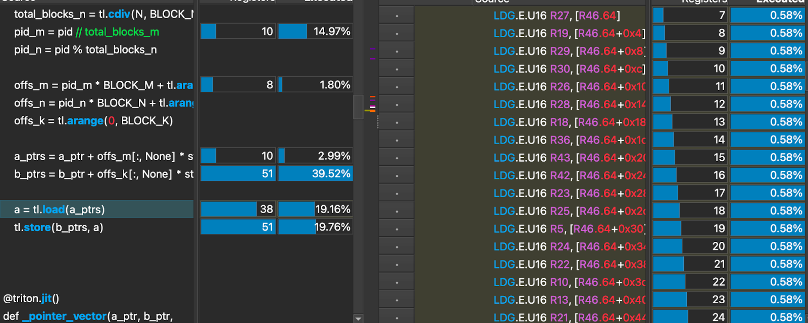
This load operation resulted in 32 global load operations that are 16 bit wide. This is not optimal.
We would like to do our global memory loads in a vectorized way so that it results in the least amount of load instructions. To combat this we can give the Triton Compiler some help.
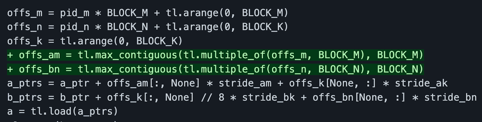
The green highlighted lines above act as a compiler hint. It tells the compiler that these elements are contiguous in memory and that this load operation can be coalesced.
Let’s see the effect in assembly after adding these lines.
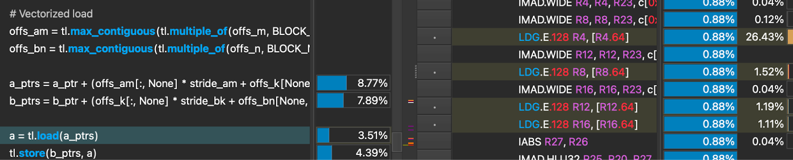
The load is now performed in 4 global load operations that are each 128 bit wide, instead of 32 16 bit global load operations. This means 28 fewer memory fetch instructions, and importantly a coalesced memory access. This can be seen from the fact that a single thread is not accessing consecutive memory addresses, which without the compiler hint, was the behavior.
The resulting effect is 73x speedup in an isolated load operation, and after incorporating it in the full dequantization kernel we were able to see another 6% speedup. Another step in the right direction!
5.0 Warp Stalling
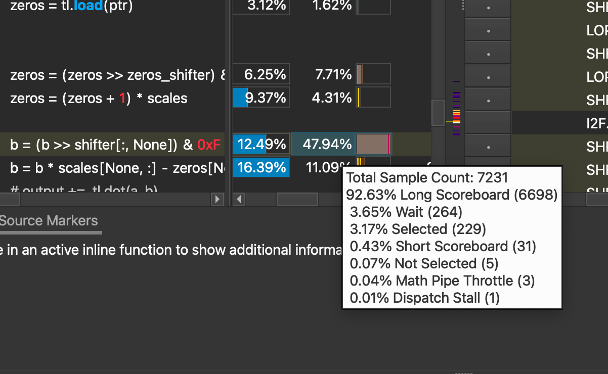
Now putting all the changes back into our full dequantization kernel, we see the following performance limiter, warp stalling.
These warp stalls are mostly caused by ‘Long Scoreboard’ stalls, accounting for 92.63% of the total.
At a high level, long scoreboard stalls happen when a warp requires data that may not be ready yet in order to be in the “issued” state. In other words GPUs are throughput machines, and we need to hide the latency of load instructions with compute instructions. By loading more data and rearranging where the load instructions are in the script we can take care of this problem.
In an ideal scenario, each warp scheduler would be able to issue 1 instruction every clock cycle. Note – Every SM on an A100 GPU has 4 warp schedulers.
However – our kernel has bottlenecks and is spending 4.4 cycles in the stall state with the block size that AutoGPTQ Triton kernel deems as optimal given the presets it has.
How do we improve this?
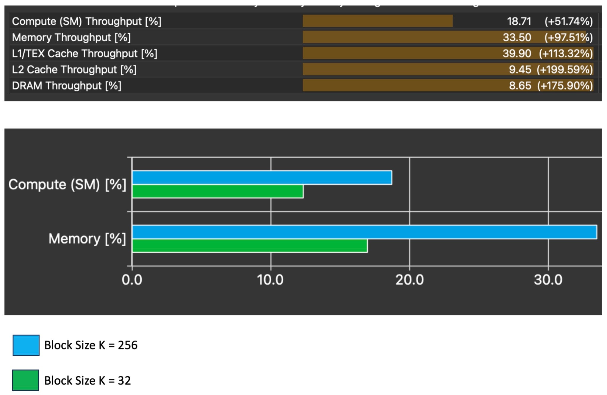
We want to be able to increase our memory throughput so that we can increase the chance that when a warp issues an instruction, we won’t be waiting for loads to be stored in SRAM so that they can be used for computation. We played around with multiple parameters (such as number of pipeline stages, and number of warps) and the one that had the biggest impact was increasing the block size by a factor of 2 in the k dimension.
These changes yield an immediate impact on both compute and memory throughput.
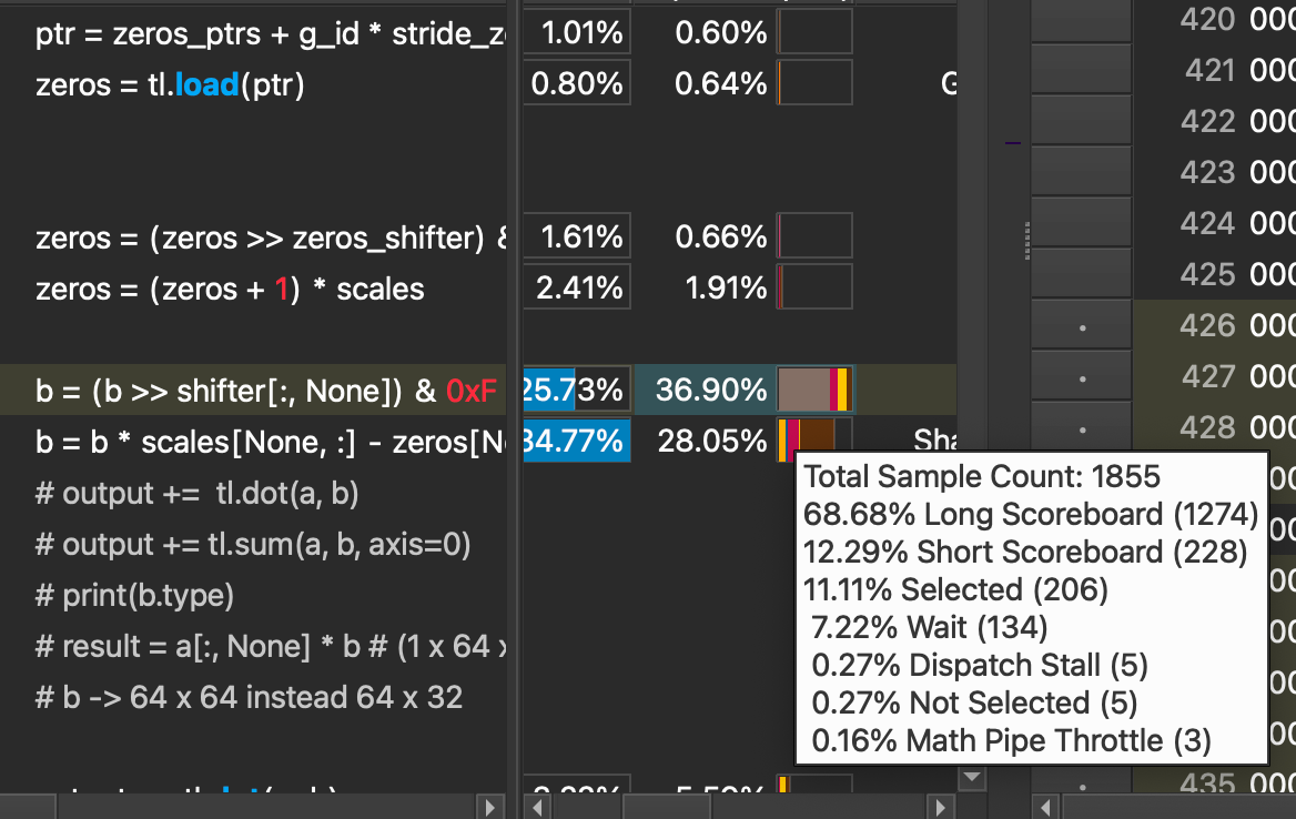
We also see the long scoreboard wait time at the step where we shift and scale the quantized weights drop significantly, which is what we identified as the original bottleneck in the source code. While there are still stalls at this line, only 68% of them are caused by long scoreboard stalls, compared to the original 92%. Ideally, we do not observe ANY stalls, so there is still work to be done here, but a reduction in the amount of stalls caused by long scoreboard tells us that our data is at this point ready to be used (in L1TEX) memory by an instruction that a warp wants to execute, at a higher frequency then the original kernel.
The corresponding impact is a 1.4x speedup in the execution time of our kernel.
6.0 Results
By tackling all these problem areas methodically our resulting kernel is 6x faster on the Nvidia A100 GPU than if you were to use the Triton kernel AutoGPTQ provides out-of-the-box.
Taking a relevant Llama inference sample data point, the Triton kernel we’ve developed takes 47us to perform dequantization and matrix multiplication compared to the 275us taken by the AutoGPTQ kernel for the same matrix size.
By replicating this step-by-step approach it should be possible to get similar speedups in other kernels, and help build understanding on common GPU bottlenecks and how to tackle them.
It is important to note that while strides have been made in improving the performance of the AutoGPTQ Triton Kernel, we have still not closed the gap on the current exllamaV2 CUDA kernels found in AutoGPTQ.
More research is required to understand how we can further optimize this kernel to match equivalent custom CUDA kernel performance.
Summary and Future work
Triton extends PyTorch by allowing low level GPU optimizations to be done at a higher level of abstraction than CUDA programming, with the net result that adding optimized Triton kernels can help PyTorch models run faster.
Our goal in this post was to show an example of accelerating the GPTQ dequant kernel and provide a template workflow for how the accelerations were achieved.
For future work, SplitK work decomposition for the matrix multiplication is a potential speed up we’ll investigate.
Integrating custom Triton Kernels into PyTorch
Given the acceleration shown above, a common question is how to actually use a custom kernel in a given PyTorch codebase.
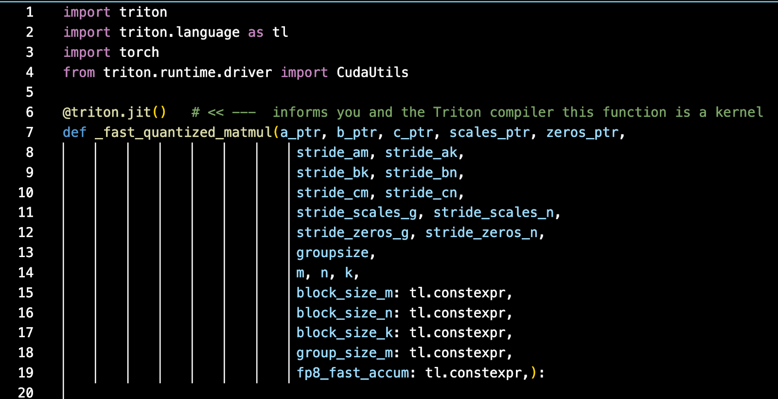
A triton kernel will contain at least two parts – the actual Triton kernel code which will be compiled by the Triton compiler:
Along with the actual kernel code is a python wrapper, that may or may not subclass the PyTorch autograd class – depending if it’s going to support a backwards pass (i.e. for training purposes or only for inference purposes).
You simply import the python class into your PyTorch code where you want to use it much like any other Python / PyTorch function.
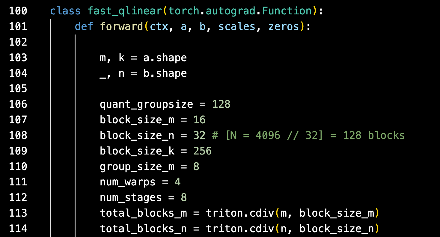
In this case, simply importing and then using ‘fast_qlinear’ would invoke the underlying Triton kernel with the speed-ups we’ve shown above applied to your PyTorch model.
Acknowledgements
Thanks to Jamie Yang and Hao Yu from IBM Research for their technical guidance in the collection of these results.