This post is the first part of a multi-series blog focused on how to accelerate generative AI models with pure, native PyTorch. We are excited to share a breadth of newly released PyTorch performance features alongside practical examples of how these features can be combined to see how far we can push PyTorch native performance.
As announced during the PyTorch Developer Conference 2023, the PyTorch team rewrote Meta’s Segment Anything (“SAM”) Model resulting in 8x faster code than the original implementation, with no loss of accuracy, all using native PyTorch optimizations. We leverage a breadth of new PyTorch features:
- Torch.compile: A compiler for PyTorch models
- GPU quantization: Accelerate models with reduced precision operations
- Scaled Dot Product Attention (SDPA): Memory efficient attention implementations
- Semi-Structured (2:4) Sparsity: A GPU optimized sparse memory format
- Nested Tensor: Batch together non-uniformly sized data into a single Tensor, such as images of different sizes.
- Custom operators with Triton: Write GPU operations using Triton Python DSL and easily integrate it into PyTorch’s various components with custom operator registration.
We encourage readers to copy-paste code from our implementation of SAM on Github and ask us questions on Github.
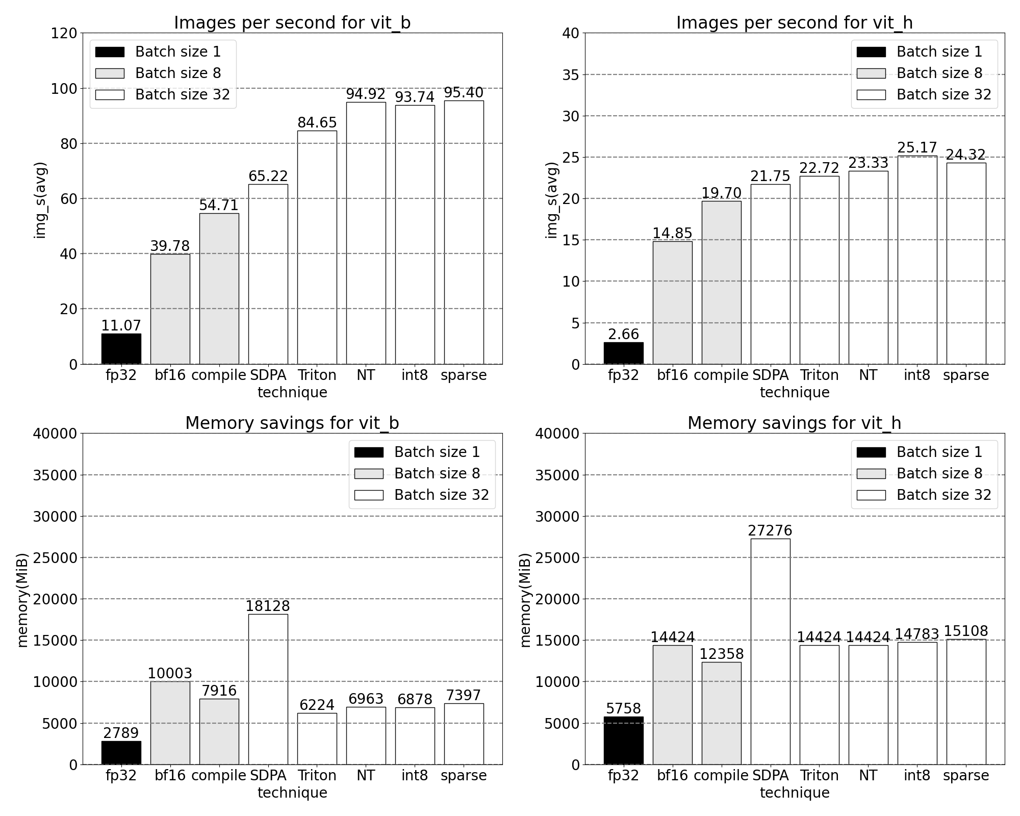
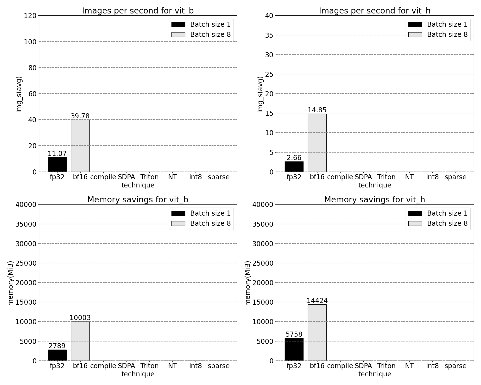
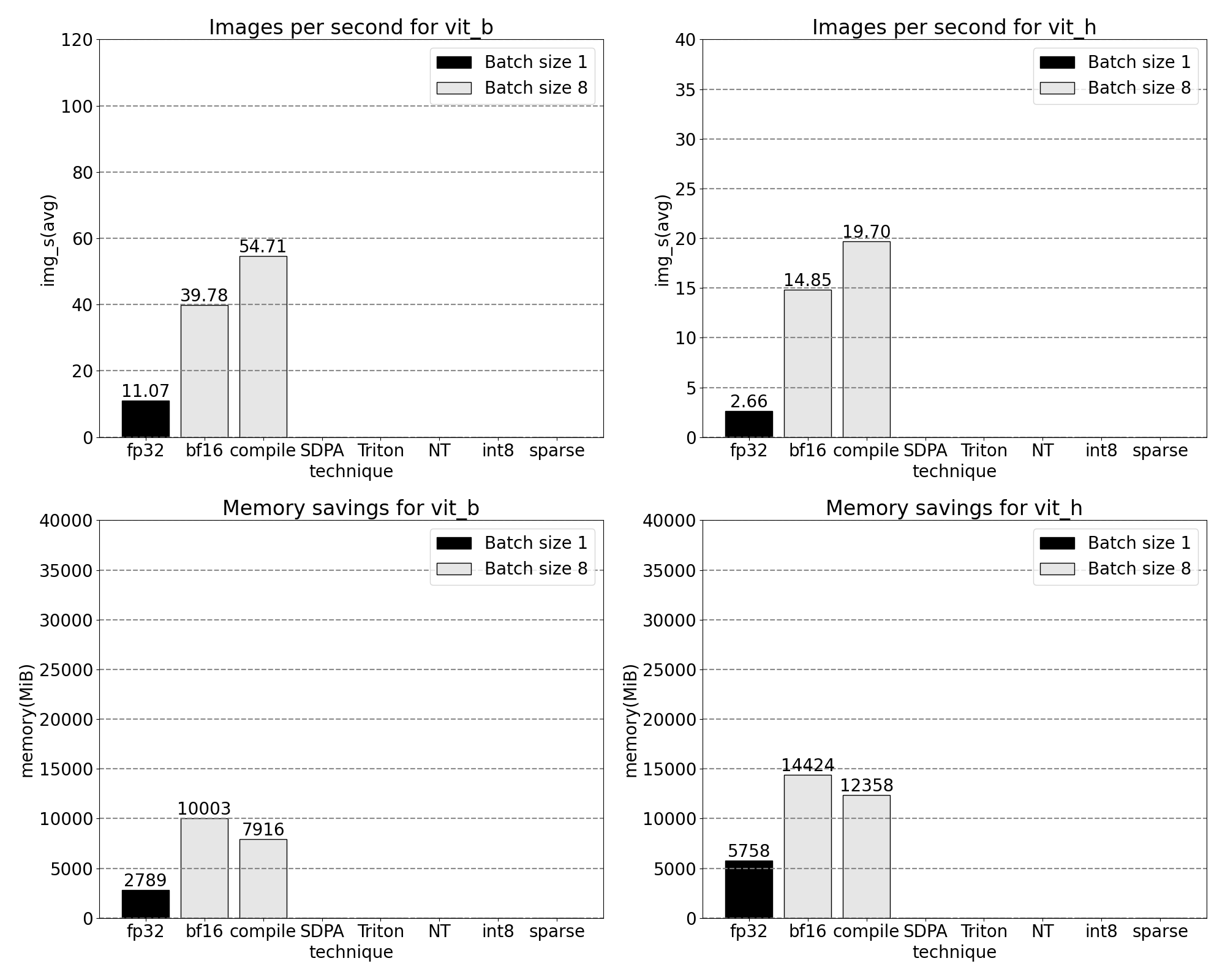
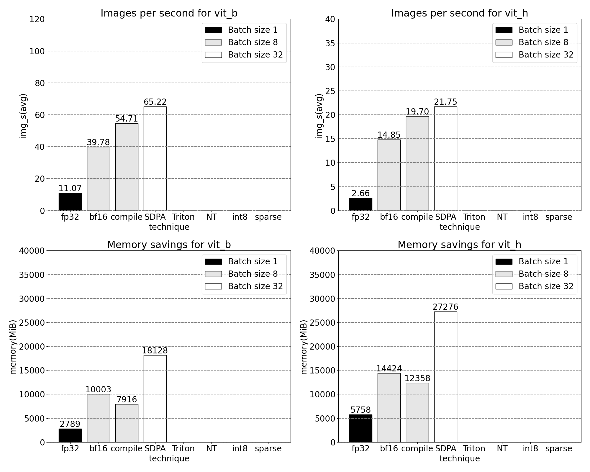
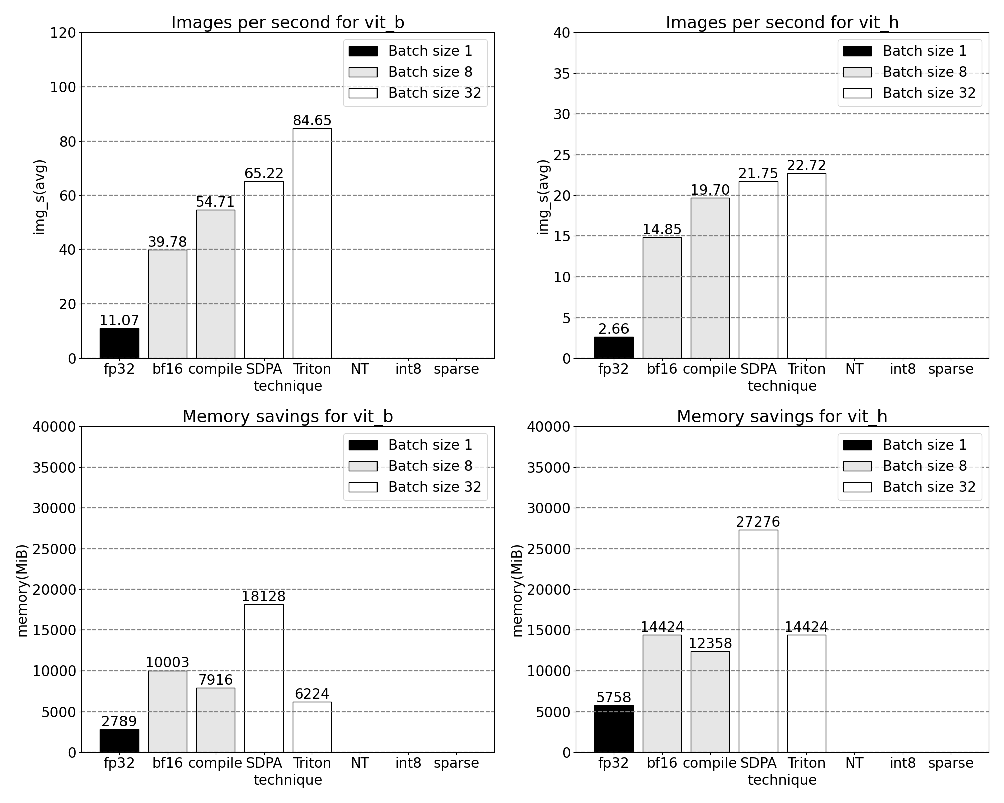
A quick glimpse of increasing throughput and decreasing memory overhead with our newly released, PyTorch native, features. Benchmarks run on p4d.24xlarge instance (8x A100s).
SegmentAnything Model
SAM is a zero-shot vision model for generating promptable image masks.

The SAM architecture [described in its paper] includes multiple prompt and image encoders based on the Transformer architecture. Of this, we measured performance across the smallest and largest vision transformer backbones: ViT-B and ViT-H. And for simplicity, we only show traces for the ViT-B model.
Optimizations
Below we tell the story of optimizing SAM: profiling, identifying bottlenecks, and building new features into PyTorch that solve these problems. Throughout, we showcase our new PyTorch features: torch.compile, SDPA, Triton kernels, Nested Tensor and semi-structured sparsity. The following sections are progressively built upon each other, ending with our SAM-fast, now available on Github. We motivate each feature using real kernel and memory traces, using fully PyTorch native tooling, and visualize these traces with Perfetto UI.
Baseline
Our SAM baseline is Facebook Research’s unmodified model, using float32 dtype and a batch size of 1. After some initial warmup, we can look at a kernel trace using the PyTorch Profiler:
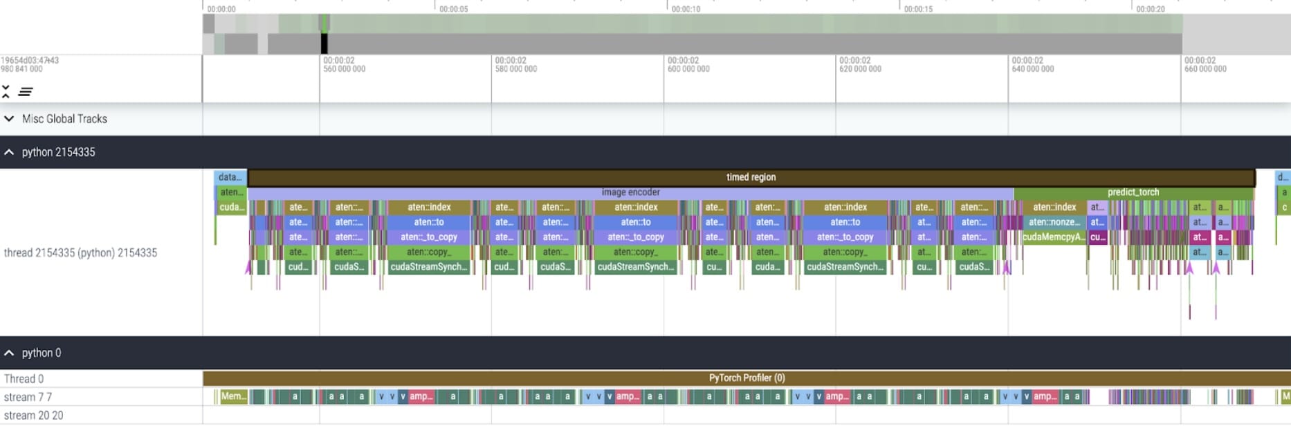
We notice two areas ripe for optimization.
The first is long calls to aten::index, the underlying call resulting from a Tensor index operation (e.g., []). While the actual GPU time spent on aten::index is relatively low. aten::index is launching two kernels, and a blocking cudaStreamSynchronize is happening in between. This means the CPU is waiting for the GPU to finish processing until it launches the second kernel. To optimize SAM, we should aim to remove blocking GPU syncs causing idle time.
The second is significant time spent on GPU in matrix multiplication (dark green on stream 7 7 above). This is common in Transformers. We can significantly speed up SAM if we can reduce the amount of GPU time spent on matrix multiplication.
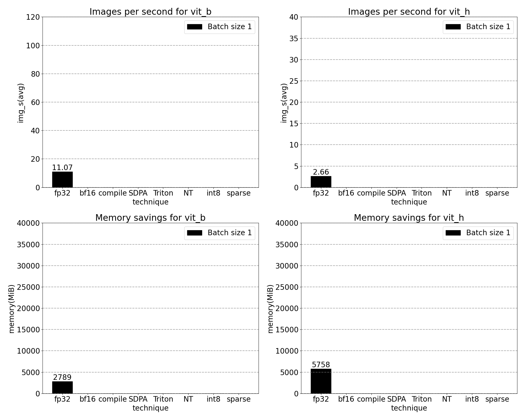
We can measure the throughput (img/s) and memory overhead (GiB) from out of the box SAM to establish a baseline:
Bfloat16 Half precision (+GPU syncs and batching)
To address the first issue of less time spent in matrix multiplication, we can turn to bfloat16. Bfloat16 is a commonly used half-precision type. Through less precision per parameter and activations, we can save significant time and memory in computation. With reducing precision of parameters, it’s critical to validate end to end model accuracy.
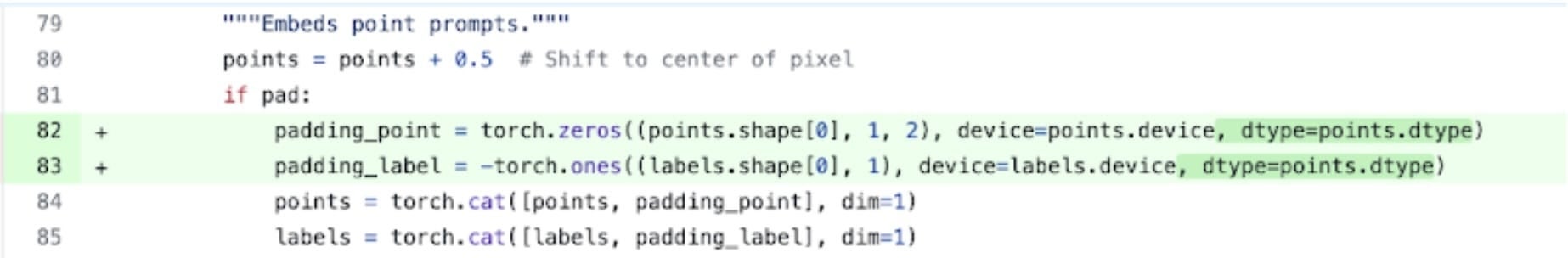
Shown here is an example of replacing padding dtypes with half precision, bfloat16. Code is here.
Next to simply setting model.to(torch.bfloat16) we have to change a few small places that assume the default dtype.
Now, in order to remove GPU syncs we need to audit operations that cause them. We can find these pieces of code by searching the GPU traces for calls to cudaStreamSynchronize. In fact, we found two locations that we were able to rewrite to be sync-free.
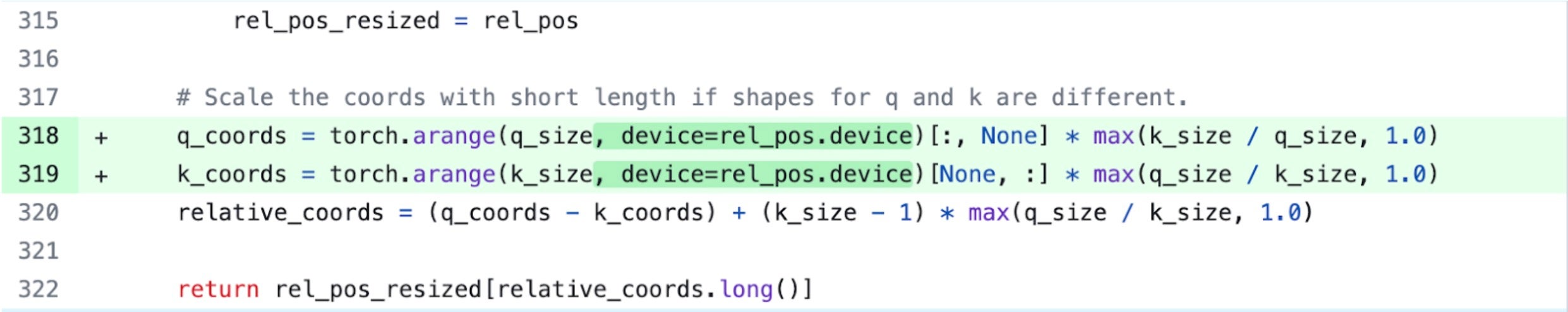
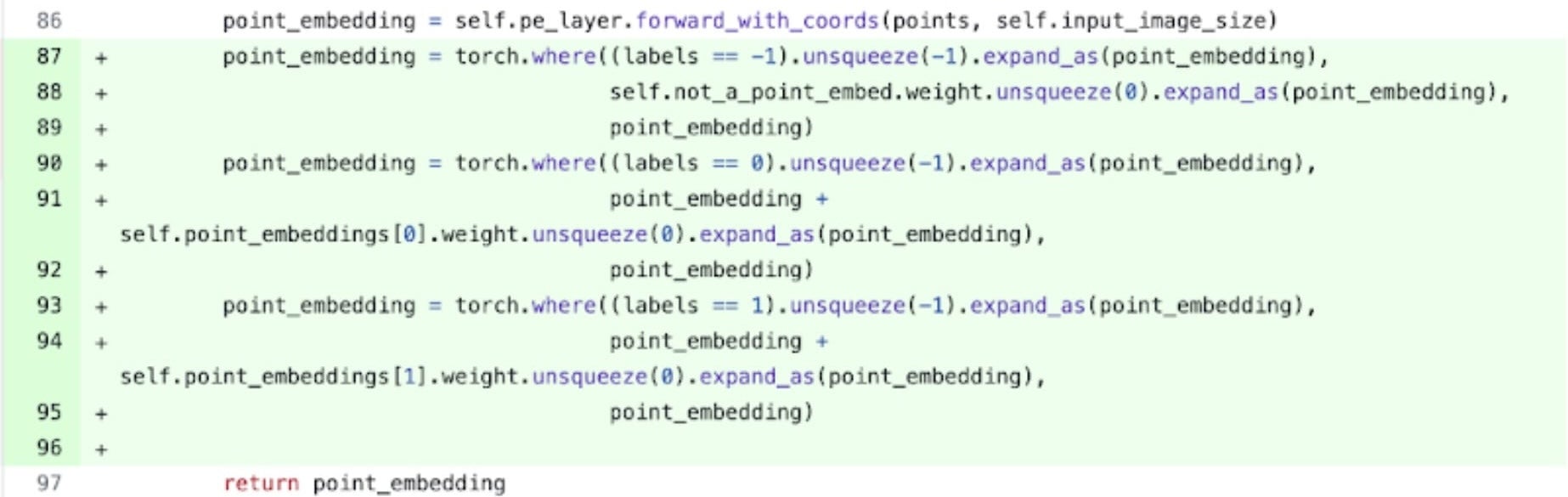
Specifically, we see that within SAM’s image encoder, there are variables acting as coordinate scalers, q_coords and k_coords. These are both allocated and processed on the CPU. However, once these variables are used to index in rel_pos_resized, the index operation automatically moves these variables to the GPU. This copy over causes the GPU sync we’ve observed above. We notice a second call to index in SAM’s prompt encoder: We can use torch.where to rewrite this as shown above.
Kernel trace
After applying these changes, we begin to see significant time between individual kernel calls. This is typically observed with small batch sizes (1 here) due to the GPU overhead of launching kernels. To get a closer look at practical areas for optimization, we can start to profile SAM inference with batch size 8:

Looking at the time spent per-kernel, we obverse most of SAM’s GPU time spent on elementwise kernels and softmax operation. With this we now see that matrix multiplications have become a much smaller relative overhead.
Taken the GPU sync and bfloat16 optimizations together, we have now pushed SAM performance by up to 3x
Torch.compile (+graph breaks and CUDA graphs)
When observing a large number of small operations, such as the elementwise kernels profiled above, turning to a compiler to fuse operations can have strong benefits. PyTorch’s recently released torch.compile does a great job optimizing by:
- Fusing together sequences of operations such as nn.LayerNorm or nn.GELU into a single GPU kernel that is called and
- Epilogues: fusing operations that immediately follow matrix multiplication kernels to reduce the number of GPU kernel calls.
Through these optimizations, we reduce the number of GPU global memory roundtrips, thus speeding up inference. We can now try torch.compile on SAM’s image encoder. To maximize performance we use a few advanced compile techniques such as:
- using torch.compile’s max-autotune mode enables CUDA graphs and shape-specific kernels with custom epilogues
- By setting TORCH_LOGS=”graph_breaks,recompiles” we can manually verify that we are not running into graph breaks or recompiles.
- Padding the batch of images input to the encoder with zeros ensures compile accepts static shapes thus being able to always use shape-specific optimized kernels with custom epilogues without recompilations.
predictor.model.image_encoder = \
    torch.compile(predictor.model.image_encoder, mode=use_compile)
Kernel trace
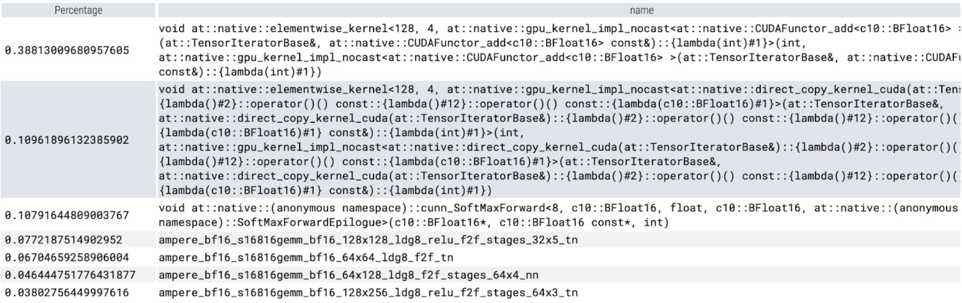
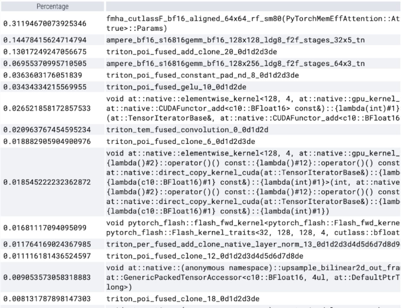
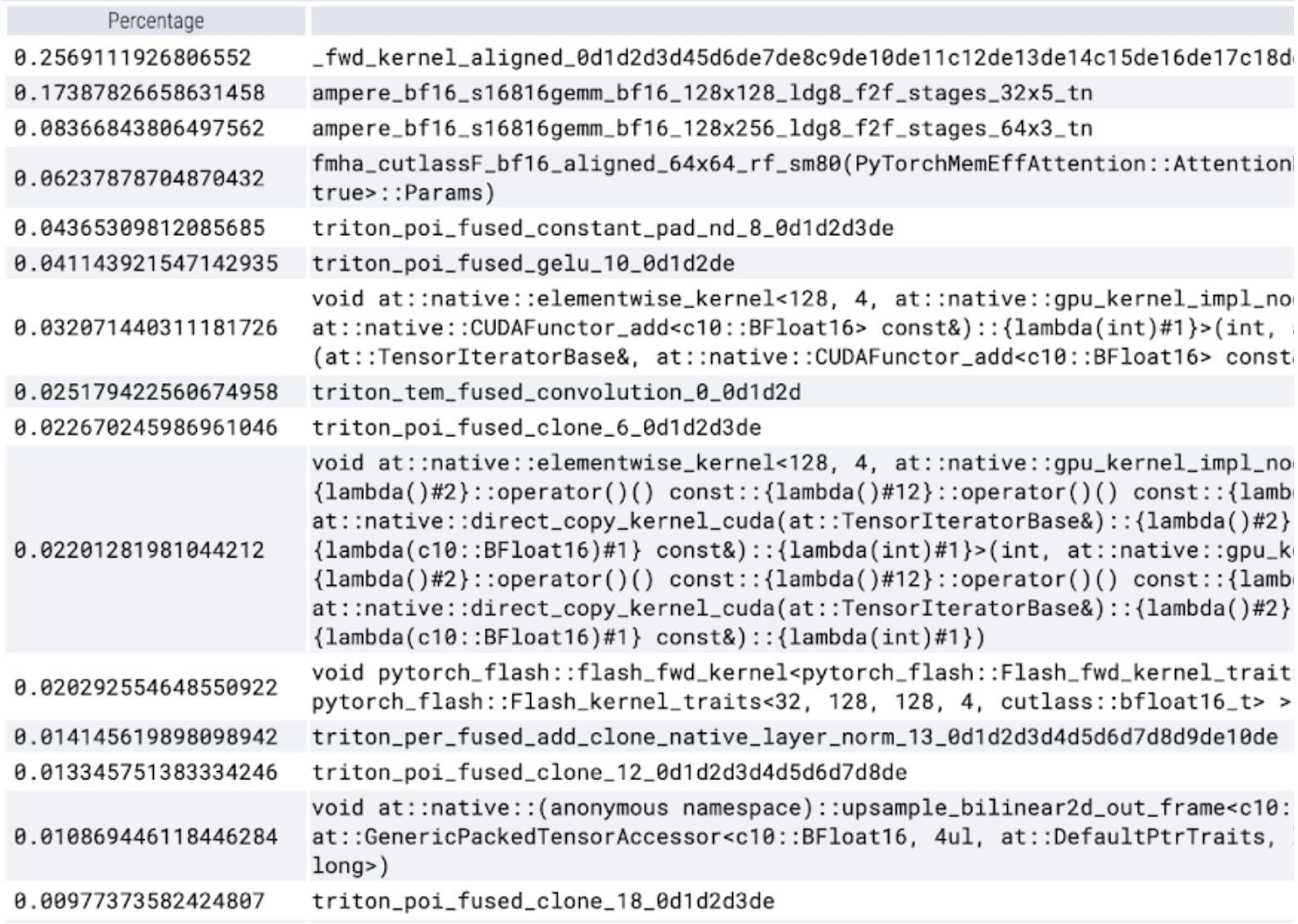
torch.compile is working beautifully. We launch a single CUDA graph, which makes up a significant portion of GPU time within the timed region. Let’s run our profile again and look at the percentage of GPU time spent in specific kernels:
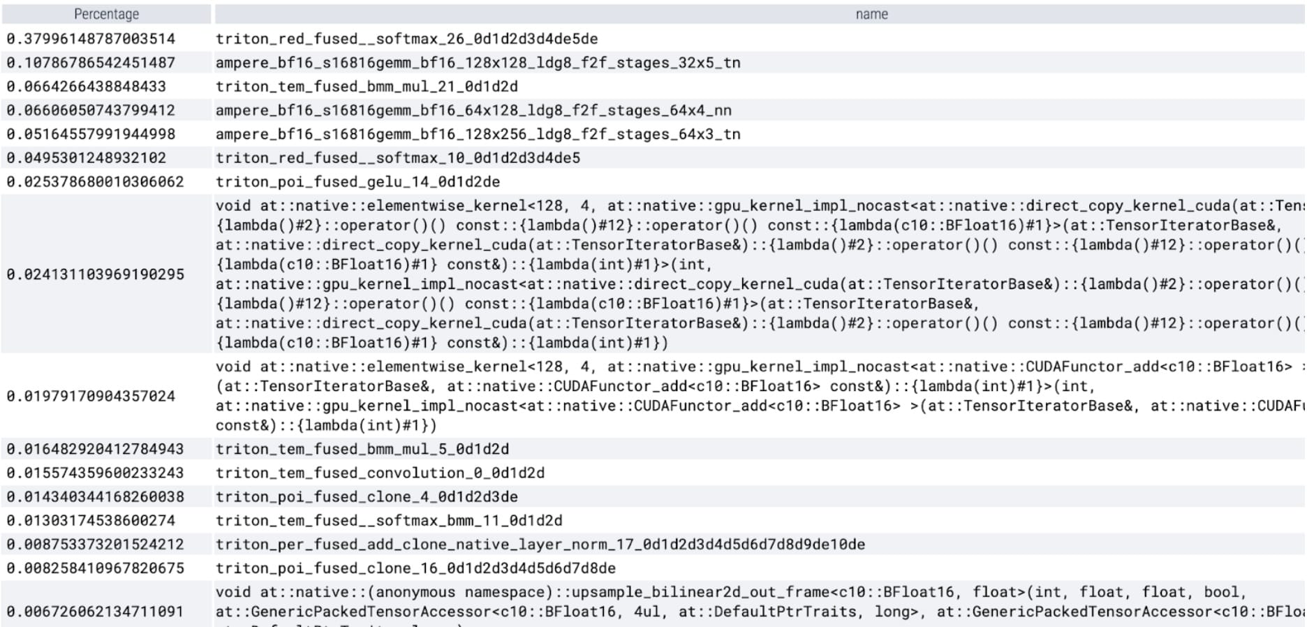
We now see softmax makes up a significant portion of the time followed by various GEMM variants. In summary we observe the following measurements for batch size 8 and above changes.
SDPA: scaled_dot_product_attention
Next up, we can tackle one of the most common areas for transformer performance overhead: the attention mechanism. Naive attention implementations scale quadratically in time and memory with sequence length. PyTorch’s scaled_dot_product_attention operation built upon the principles of Flash Attention, FlashAttentionV2 and xFormer’s memory efficient attention can significantly speed up GPU attention. Combined with torch.compile, this operation allows us to express and fuse a common pattern within variants of MultiheadAttention. After a small set of changes we can adapt the model to use scaled_dot_product_attention.
PyTorch native attention implementation, see code here.
Kernel trace
We can now see that in particular the memory efficient attention kernel is taking up a large amount of computational time on the GPU:
Using PyTorch’s native scaled_dot_product_attention, we can significantly increase the batch size. We now observe the following measurements for batch size 32 and above changes.
Triton: Custom SDPA for fused relative positional encoding
Transitioning away from inference throughput for a moment, we started profiling overall SAM memory. Within the image encoder, we saw significant spikes in memory allocation:
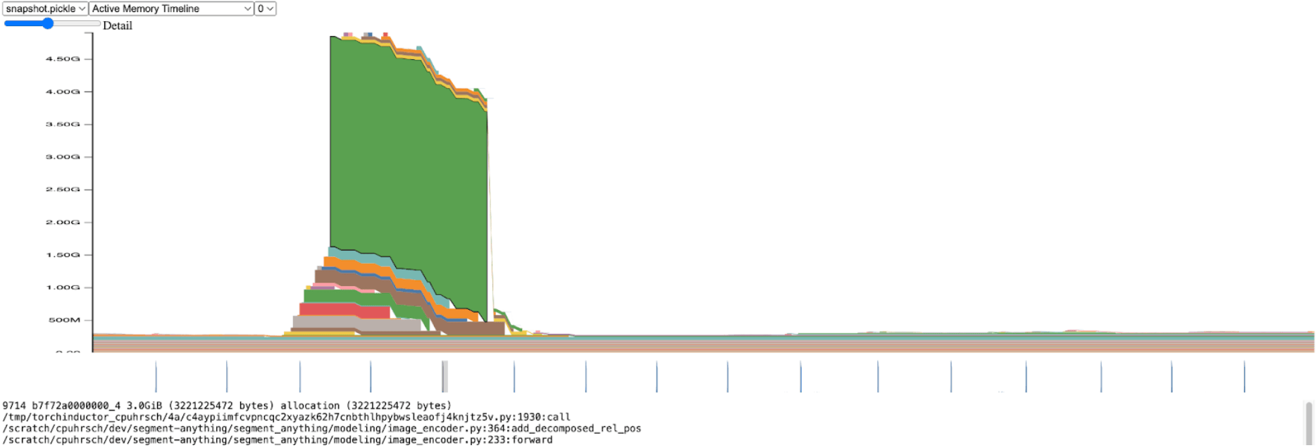
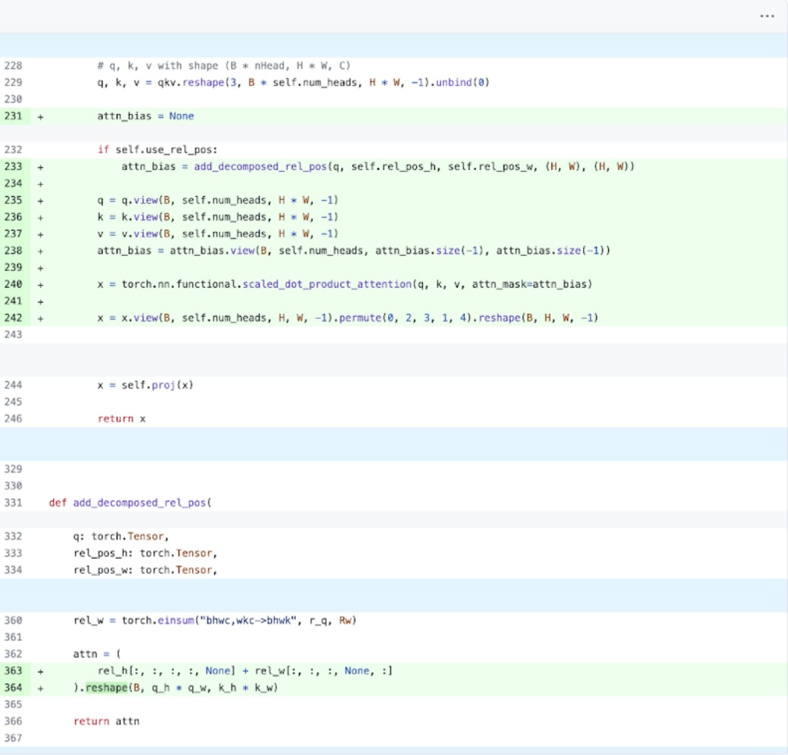
Zooming in, we see this allocation happens within add_decomposed_rel_pos, on the following line:
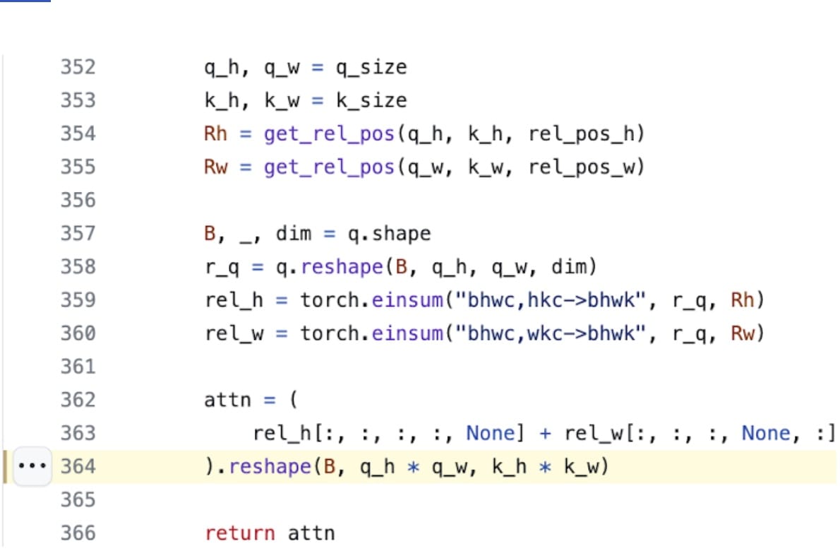
The attn variable here is the addition of two smaller tensors: rel_h of shape (B, q_h, q_w, k_h, 1) and rel_w of shape (B, q_h, q_w, 1, k_w).
It’s not surprising that the memory efficient attention kernel (used via SDPA) is taking a long time with an attention bias size over 3.0GiB. If instead of allocating this large attn tensor, we thread into SDPA the two smaller rel_h and rel_w tensors, and only construct attn as needed, we’d anticipate significant performance gain.
Unfortunately this is not a trivial modification; SDPA kernels are highly optimized and written in CUDA. We can turn to Triton, with their easy to understand and use tutorial on a FlashAttention implementation. After some significant digging and in close collaboration with xFormer’s Daniel Haziza we found one case of input shapes where it is relatively straightforward to implement a fused version of the kernel. The details have been added to the repository. Surprisingly this can be done in under 350 lines of code for the inference case.
This is a great example of extending PyTorch with a new kernel, straightforwardly built with Triton code.
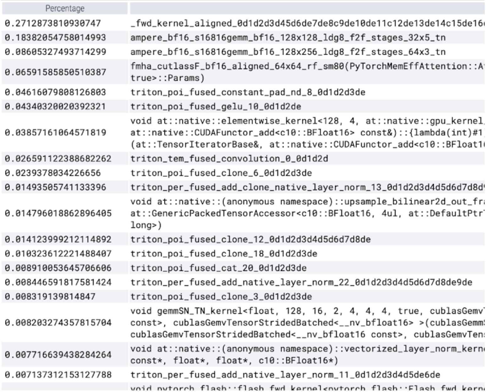
Kernel trace
With our custom positional Triton kernel we observe the following measurements for batch size 32.
NT: NestedTensor and batching predict_torch
We have spent a lot of time on the image encoder. This makes sense, since it takes up the most amount of computational time. At this point however it is fairly well optimized and the operator that takes the most time would require significant additional investment to be improved.
We discovered an interesting observation with the mask prediction pipeline: for each image we have there is an associated size, coords, and fg_labels Tensor. Each of these tensors are of different batch sizes. Each image itself is also of a different size. This representation of data looks like Jagged Data. With PyTorch’s recently released NestedTensor, we can modify our data pipeline batch coords and fg_labels Tensors into a single NestedTensor. This can have significant performance benefits for the prompt encoder and mask decoder that follow the image encoder. Invoking:
torch.nested.nested_tensor(data, dtype=dtype, layout=torch.jagged)
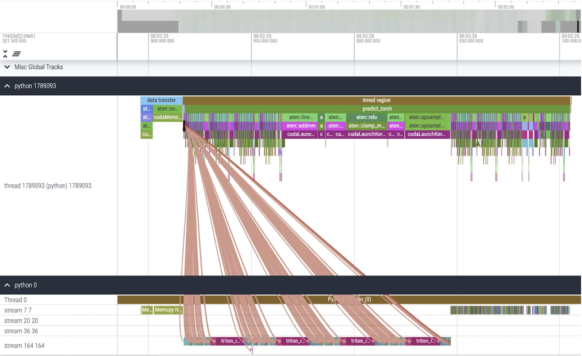
Kernel trace
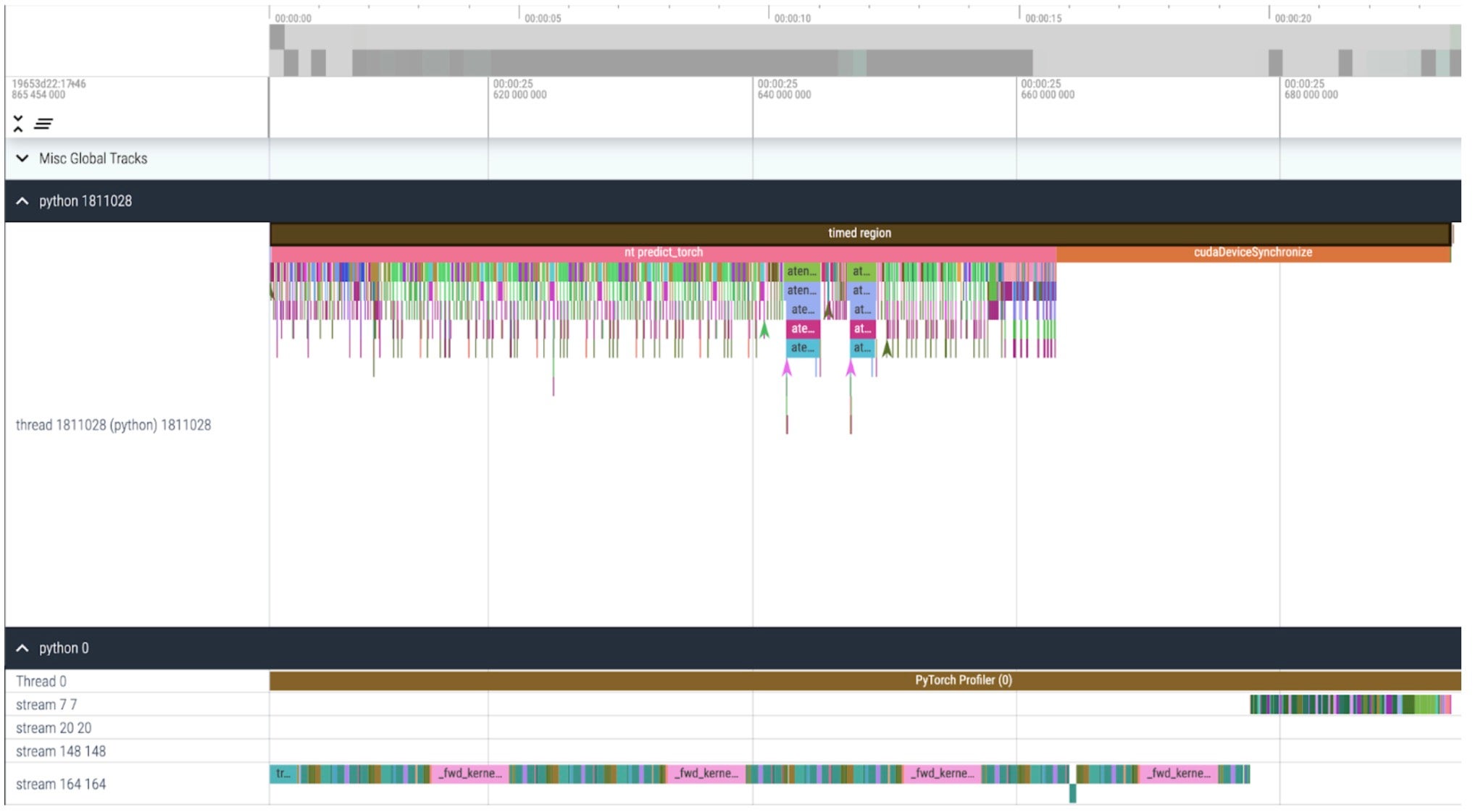
We can see now that we can launch kernels much faster from the CPU than the GPU can process and that it spends a long time waiting at the end of our timed region for the GPU to finish (cudaDeviceSynchronize). We also don’t see any more idle time (white space) between kernels on the GPU.
With Nested Tensor, we observe the following measurements for batch size 32 and above changes.
int8: quantization and approximating matmul
We notice in the above trace, that significant time is now spent in GEMM kernels. We’ve optimized enough that we now see matrix multiplication account for more time in inference than scaled dot product attention.
Building on earlier learnings going from fp32 to bfloat16, let’s go a step further, emulating even lower precision with int8 quantization. Looking at quantization methods, we focus on Dynamic quantization wherein our model observes the range of possible inputs and weights of a layer, and subdivides the expressible int8 range to uniformly “spread out” observed values. Ultimately each float input will be mapped to a single integer in the range [-128, 127]. For more information see PyTorch’s tutorial on quantization
Reducing precision can immediately lead to peak memory savings, but to realize inference speedups, we have to make full use of int8 through SAM’s operations. This requires building an efficient int8@int8 matrix multiplication kernel, as well as casting logic to translate from high to low precision (quantization) as well as reversing back from low to high (dequantization). Utilizing the power of torch.compile, we can compile and fuse together these quantization and dequantization routines into efficient single kernels and epilogues of our matrix multiplication. The resulting implementation is fairly short and less than 250 lines of code. For more information on the APIs and usage, see pytorch-labs/ao.
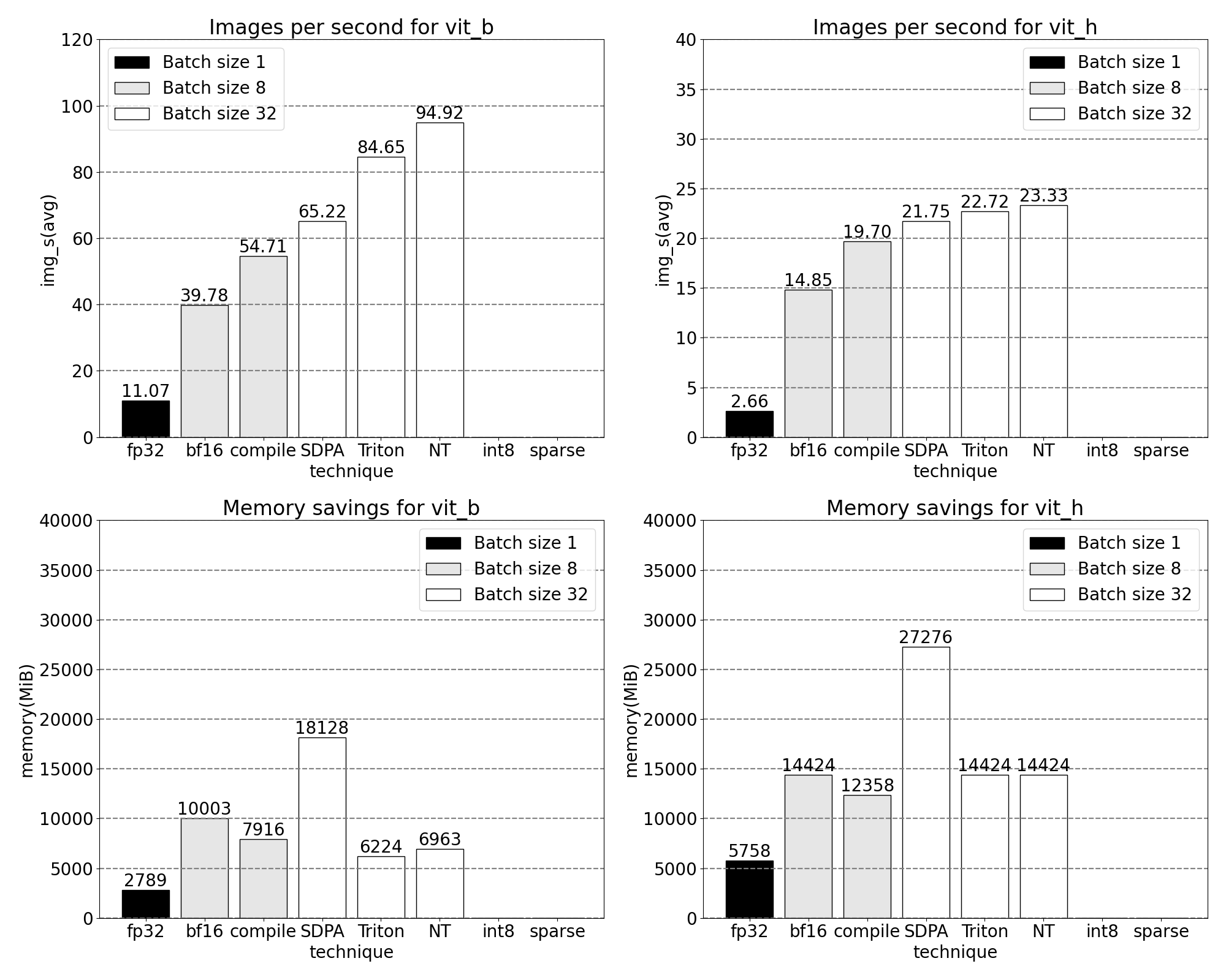
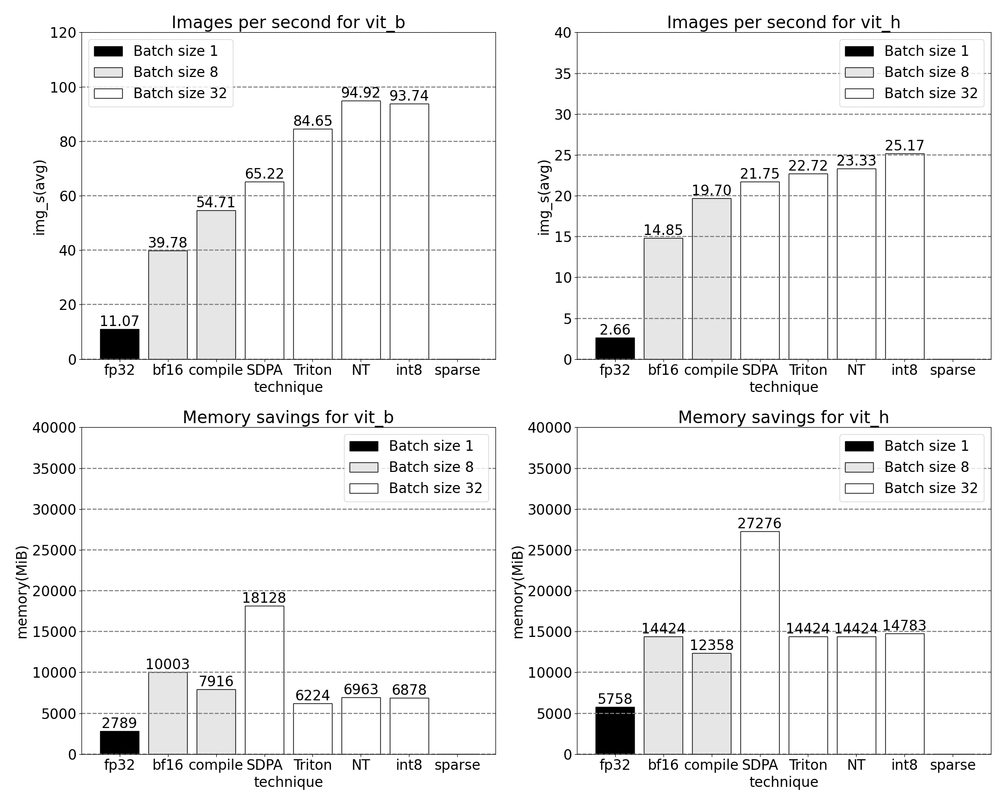
While it’s common to see some accuracy regression when quantizing models at inference time, SAM has been particularly robust to lower precision inference with minimal loss of accuracy. With quantization added, we now observe the following measurements for batch size 32 and above changes.
sparse: Semi-structured (2:4) sparsity
Matrix multiplications are still our bottleneck. We can turn to the model acceleration playbook with another classic method to approximate matrix multiplication: sparsification. By sparsifying our matrices (i.e., zeroing out values), we could theoretically use fewer bits to store weight and activation tensors. The process by which we decide which weights in the tensor to set to zero is called pruning. The idea behind pruning is that small weights in a weight tensor contribute little to the net output of a layer, typically the product of weights with activations. Pruning away small weights can potentially reduce model size without significant loss of accuracy.
Methods for pruning are varied, from completely unstructured, wherein weights are greedily pruned to highly structured, wherein large sub-components of a tensor are pruned a time. Choice of method is not trivial. While unstructured pruning may have the theoretically least impact on accuracy, GPUs are also highly efficient with multiplying large, dense matrices and may suffer significant performance degradation in sparse regimes. One recent pruning method supported in PyTorch seeks to strike a balance, called semi-structured (or 2:4) sparsity. This sparse storage reduces the original tensor by a significant 50%, while simultaneously resulting in a dense tensor output that can leverage highly performant, 2:4 GPU kernels. See the following picture for an illustration.
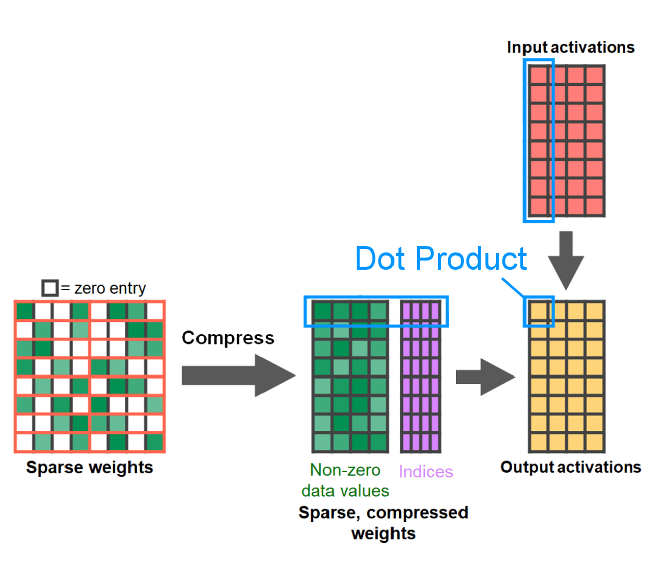
From developer.nvidia.com/blog/exploiting-ampere-structured-sparsity-with-cusparselt
In order to use this sparse storage format and the associated fast kernels we need to prune our weights such that they adhere to the constraints for the format. We pick the two smallest weights to prune in a 1 by 4 region, measuring the performance vs accuracy tradeoff. It is easy to change a weight from its default PyTorch (“strided”) layout to this new, semi-structured sparse layout. To implement apply_sparse(model) we only require 32 lines of Python code:
import torch
from torch.sparse import to_sparse_semi_structured, SparseSemiStructuredTensor

# Sparsity helper functions
def apply_fake_sparsity(model):
    """
    This function simulates 2:4 sparsity on all linear layers in a model.
    It uses the torch.ao.pruning flow.
    """
    # torch.ao.pruning flow
    from torch.ao.pruning import WeightNormSparsifier
    sparse_config = []
    for name, mod in model.named_modules():
        if isinstance(mod, torch.nn.Linear):
            sparse_config.append({"tensor_fqn": f"{name}.weight"})

    sparsifier = WeightNormSparsifier(sparsity_level=1.0,
                                      sparse_block_shape=(1,4),
                                      zeros_per_block=2)
    sparsifier.prepare(model, sparse_config)
    sparsifier.step()

    sparsifier.step()
    sparsifier.squash_mask()


def apply_sparse(model):
    apply_fake_sparsity(model)
    for name, mod in model.named_modules():
        if isinstance(mod, torch.nn.Linear):
            mod.weight = torch.nn.Parameter(to_sparse_semi_structured(mod.weight))
With 2:4 sparsity, we observe peak performance on SAM with vit_b and batch size 32:
Conclusion
Wrapping up, we are excited to have announced our fastest implementation of Segment Anything to date. We rewrote Meta’s original SAM in pure PyTorch with no loss of accuracy using a breadth of newly released features:
- Torch.compile PyTorch’s native JIT compiler, providing fast, automated fusion of PyTorch operations [tutorial]
- GPU quantization accelerate models with reduced precision operations [api]
- Scaled Dot Product Attention (SDPA) a new, memory efficient implementation of Attention [tutorial]
- Semi-Structured (2:4) Sparsity accelerate models with fewer bits to store weights and activations [tutorial]
- Nested Tensor Highly optimized, ragged array handling for non-uniform batch and image sizes [tutorial]
- Triton kernels. Custom GPU operations, easily built and optimized via Triton
For more details on how to reproduce the data presented in this blog post, check out the experiments folder of segment-anything-fast. Please don’t hesitate to contact us or open an issue if you run into any technical issues.
In our next post, we are excited to share similar performance gains with our PyTorch natively authored LLM!
Acknowledgements
We would like to thank Meta’s xFormers team including Daniel Haziza and Francisco Massa for authoring SDPA kernels and helping us design our custom one-off Triton kernel.